nf-core/proteinfold
Protein 3D structure prediction pipeline
Introduction
This document describes the user-facing output produced by the pipeline.
Pipeline overview
The pipeline is built using Nextflow and predicts protein structures using the following methods:
See main README.md for a condensed overview of the steps in the pipeline, and the bioinformatics tools used at each step.
The directories listed below will be created in the output directory after the pipeline has finished. All paths are relative to the top-level results directory.
Exact subdirectories depend on the selected mode(s). In a multi-mode run (for example alphafold2,boltz,rosettafold_all_atom) you will typically see top-level directories such as alphafold2/, boltz/, rosettafold_all_atom/, multiqc/, reports/, compare/, and pipeline_info/.
Prediction outputs (all modes)
User-facing outputs are largely consistent across modes.
Common output patterns
<MODE>/top_ranked_structures/<SEQUENCE NAME>.pdb<MODE>/<SEQUENCE NAME>/<SEQUENCE NAME>_plddt.tsv<MODE>/<SEQUENCE NAME>/paes/<SEQUENCE NAME>_<RANK>_pae.tsv(when available)<MODE>/<SEQUENCE NAME>/<SEQUENCE NAME>_<MODE>_msa.tsv(mode-specific MSA summary)<MODE>/<SEQUENCE NAME>/<SEQUENCE NAME>_{ptm,iptm}.tsvand chainwise summaries (where applicable)
pLDDT ({meta.id}_plddt.tsv)
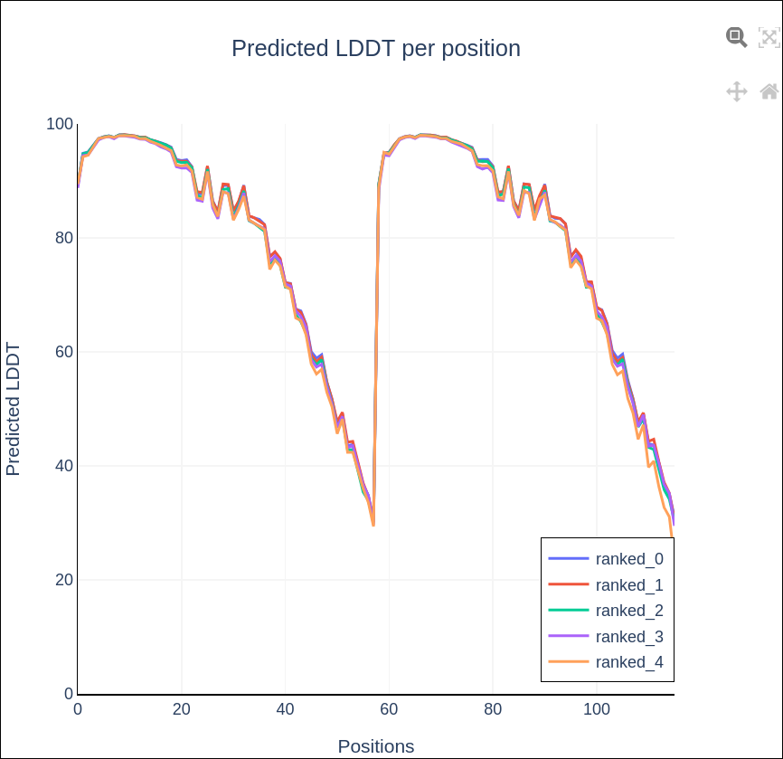
Confidence values per residue, rounded to 2 decimal places. Each ranked result gets its own column (for all-atom modules, atomic token confidences are processed to a naive mean value across the residue).
Positions	rank_0	rank_1	rank_2	rank_3	rank_4
0	83.58	85.27	88.41	86.22	84.91
1	97.99	97.81	97.39	97.49	97.32
2	98.22	98.42	98.16	97.88	97.81
3	98.06	98.15	97.94	97.56	97.4
4	98.67	98.56	98.3	98.38	98.29
5	98.81	98.77	98.62	98.61	98.54
6	98.79	98.74	98.57	98.59	98.52
...
MSA ({meta.id}_{meta.mode}_msa.tsv)
The amino acid characters are converted to integers 0-19, unknown as 20, integer 21 represents the gap character.
19	5	5	4	10	16	15	3	8	15	13	16	12	9	17	16	9	4	8	11	0	7	7	8	11	0	19	8	8	5	3
19	5	5	4	10	16	15	3	8	15	13	16	12	9	17	16	9	4	8	11	0	7	7	8	11	0	6	8	8	5	13
19	5	5	4	10	5	15	13	14	0	14	16	12	9	17	16	9	4	14	11	0	7	5	8	15	4	5	8	3	5	21
19	5	5	4	10	16	15	3	8	15	13	16	12	9	17	16	9	4	8	11	0	7	7	8	11	0	19	8	8	5	21
19	5	5	4	10	16	15	3	8	15	13	16	12	9	17	16	9	4	8	11	0	7	7	8	11	0	19	8	8	5	13
19	5	5	4	10	16	15	3	8	15	13	16	12	9	7	16	9	4	8	11	0	7	7	8	11	0	6	8	8	5	13
This allows easy sequence indentity calculation when processing as a numpy array.
(i)pTM ({meta.id}_[i]ptm.tsv)
(i)pTM scores, rounded to 3 decimal places, listed by the rank number (currently unsorted - to reflect models and seeds where appropriate).
17  0.552
22  0.529
21  0.532
20  0.541
23  0.523
3 0.606
2 0.610
4 0.606
1 0.616
0 0.617
12  0.580
9 0.588
13  0.580
11  0.583
14  0.570
15  0.565
24  0.517
16  0.560
18  0.550
19  0.550
10  0.588
5 0.600
6 0.597
7 0.596
8 0.595
chain-wise (i)pTM ({meta.id}_chainwise_[i]ptm.tsv)
(Asymmetrical) ipTM scores, rounded to 4 decimal places, with chain pair lettering as the row (X:Y), and the rank number as the column. A pTM value is a chain’s own predicted Template Modelling score so lettering will be X:X.
0	1	2
A:B	0.2880	0.2750	0.2900
B:A	0.2904	0.2801	0.2915
PAE ({meta.id}_{rank_number}_pae.tsv)
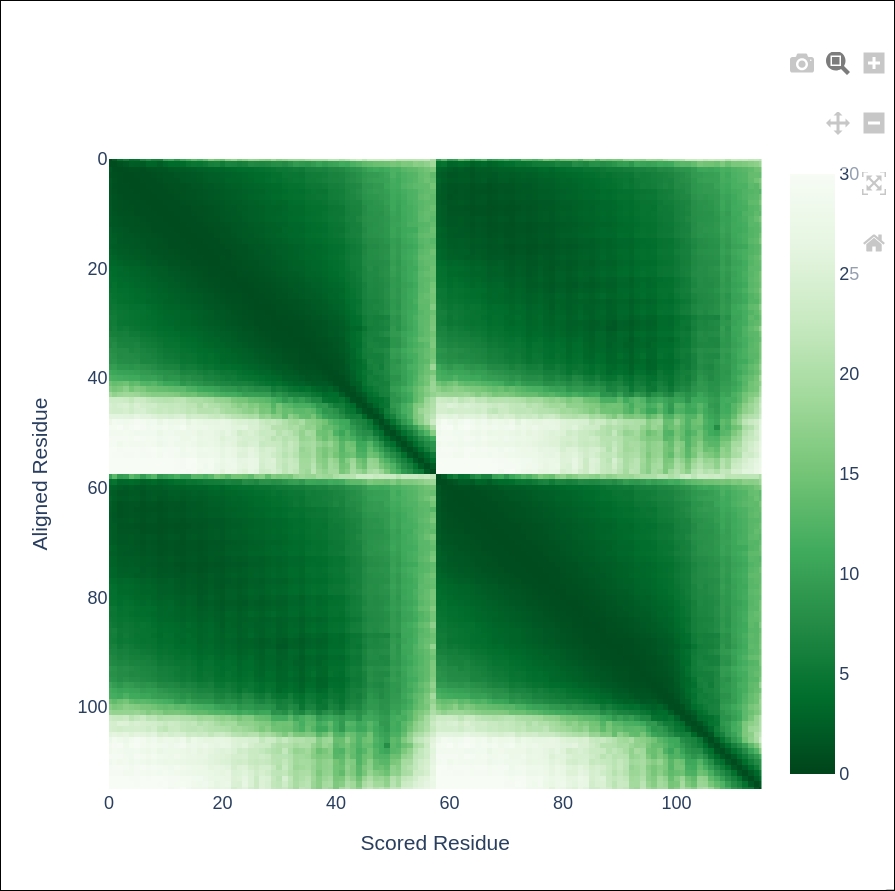
Predicted alignment error of residues j aligned by residue i, rounded to 4 decimal places.
The row number gives you the index of residue i and the column value within the row gives the index of residue j for the 2D PAE matrix.
Each model prediction generates a separate file containing the rank number. The _0_pae.tsv file corresponds to the top ranked model, other ranked results are stored within the paes/ folder.
0.2500	1.5710	3.9037	6.2177	8.4471	11.4583	12.9679	15.1237	18.0263	18.3868	18.9381	20.5747	19.3314	20.1825	21.6145	23.2190
2.2177	0.2500	1.5559	4.0327	6.3151	7.6372	10.1969	11.3626	14.9366	16.1303	17.9119	19.1877	21.2715	20.9531	20.1760	19.4087
3.4270	1.5284	0.2500	2.1333	3.5351	5.1049	6.6521	8.2317	12.1379	13.7185	14.9523	16.6154	19.6988	21.7614	18.6592	17.9619
6.1051	5.4206	2.5987	0.2500	2.0724	5.1454	6.7492	9.5538	9.6285	12.3868	13.8527	16.3586	17.2605	20.6381	19.9987	19.3295
7.3512	6.4947	5.5435	2.6740	0.2500	1.7561	4.9041	6.3923	8.9735	8.9272	12.3419	14.6005	15.9820	17.6358	20.5190	19.1028
7.4734	7.0899	5.8128	5.7512	2.0439	0.2500	1.8352	5.1064	6.4225	9.2098	10.5136	12.9404	14.3152	16.8122	18.6336	17.7382
Example report plots
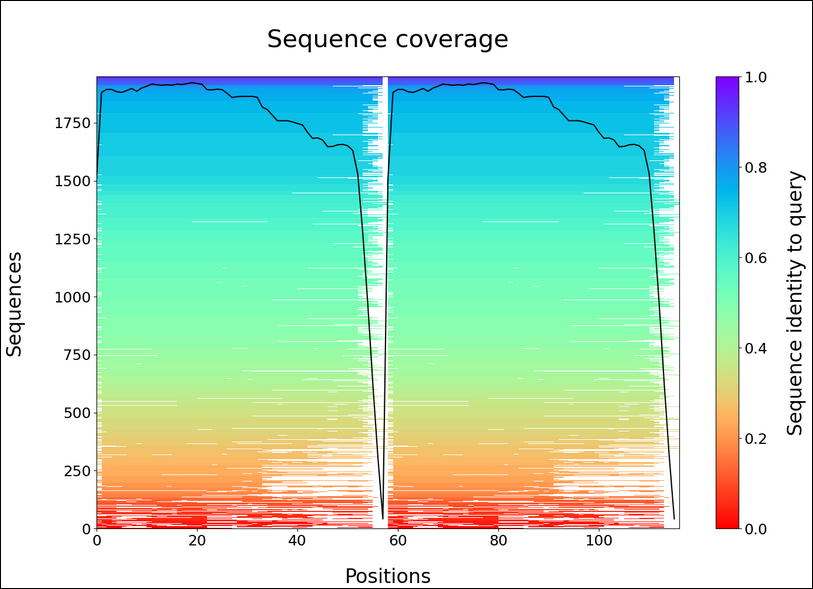
The report exports include key visualisations such as sequence coverage, predicted Local Distance Difference Test (pLDDT), and Predicted Aligned Error (PAE).
Sequence coverage

predicted Local Distance Difference Test (pLDDT)

Predicted Aligned Error (PAE)

Per-mode reports and comparisons
Output files
reports/<SEQUENCE NAME>_<MODE>_report.html(single-mode report per sequence/mode)
compare/<SEQUENCE NAME>_comparison_report.html(present when running multiple modes)
Foldseek structural similarity search
If Foldseek is enabled (--skip_foldseek false), results are written to:
Output files
foldseek_easysearch/<SEQUENCE NAME>_<MODE>_foldseek.html(default output format)<SEQUENCE NAME>.m8(tabular output when--foldseek_easysearch_argdoes not include--format-mode 3)
Foldseek runs on top-ranked structures from each selected mode and sequence. By default, the pipeline uses --format-mode 3 and publishes HTML reports.
MultiQC report
Output files
multiqc*_multiqc_report.html: Standalone HTML report(s) that can be viewed in your web browser.*_multiqc_report_data/: Parsed report data for each corresponding MultiQC report.
MultiQC is a visualisation tool that generates HTML report(s) summarising samples in your project. Most QC results are visualised in the report and further statistics are available within each corresponding *_multiqc_report_data/ directory.
Results generated by MultiQC collate QC metrics from the selected structure-prediction mode(s), and the software versions for traceability. For more information about how to use MultiQC reports, see http://multiqc.info.
Pipeline information
Output files
pipeline_info/- Reports generated by Nextflow:
execution_report.html,execution_timeline.html,execution_trace.txtandpipeline_dag.dot/pipeline_dag.svg. - Reports generated by the pipeline:
pipeline_report.html,pipeline_report.txtandsoftware_versions.yml. Thepipeline_report*files will only be present if the--email/--email_on_failparameter’s are used when running the pipeline. - Reformatted samplesheet files used as input to the pipeline:
samplesheet.valid.csv. - Parameters used by the pipeline run:
params.json.
- Reports generated by Nextflow:
Nextflow provides excellent functionality for generating various reports relevant to the running and execution of the pipeline. This will allow you to troubleshoot errors with the running of the pipeline, and also provide you with other information such as launch commands, run times and resource usage.
Additional intermediate outputs
Depending on the selected mode(s) and options, additional top-level directories may be present, for example:
fasta2yaml/(for YAML conversion inputs/outputs)mmseqs/results/(for MMseqs2 outputs such as.a3mfiles)split/output_msa/(for split-MSA intermediate CSV outputs)
--save_intermediates
If --save_intermediates is enabled, extra raw intermediate files are published in mode-specific raw/ directories.
Examples include:
alphafold2/<MODE>/<SEQUENCE NAME>/raw/colabfold/<SEQUENCE NAME>/raw/boltz/<SEQUENCE NAME>/boltz_results_*/rosettafold_all_atom/<SEQUENCE NAME>/raw/alphafold3/<SEQUENCE NAME>/raw/helixfold3/<SEQUENCE NAME>/raw/rosettafold2na/<SEQUENCE NAME>/raw/
These raw outputs are intended for advanced debugging, reproducibility and method-specific downstream analyses. For detailed, canonical tool-specific native output specifications, see: