nf-core/riboseq
Pipeline for the analysis of ribosome profiling, or Ribo-seq (also named ribosome footprinting) data.
1.0.1). The latest stable release is1.2.0.Introduction
This document describes the output produced by the pipeline. Most of the plots are taken from the MultiQC report generated from the full-sized test dataset for the pipeline using a command similar to the one below:
nextflow run nf-core/riboseq -profile test_full,<docker/singularity/institute>The directories listed below will be created in the results directory after the pipeline has finished. All paths are relative to the top-level results directory.
Pipeline overview
The pipeline is built using Nextflow and processes data using the following steps:
- Preprocessing
- cat - Merge re-sequenced FastQ files
- FastQC - Raw read QC
- UMI-tools extract - UMI barcode extraction
- TrimGalore - Adapter and quality trimming
- fastp - Adapter and quality trimming
- BBSplit - Removal of genome contaminants
- SortMeRNA - Removal of ribosomal RNA
- Ribo-TISH quality - Riboseq QC plots generated with the Ribo-TISH ‘quality’ command
- Alignment and quantification
- STAR - Fast spliced aware genome alignment
- Alignment post-processing
- SAMtools - Sort and index alignments
- UMI-tools dedup - UMI-based deduplication
- picard MarkDuplicates - Duplicate read marking
- ORF prediction - Open reading frame (ORF prediction)
- Ribo-TISH - Riboseq ORF predictions by Ribo-TISH
- Ribotricer - Riboseq QC and ORF predictions by Ribotricer
- Translational efficiency analysis
- anota2seq - Translational efficiency analysis with anota2seq
- Workflow reporting and genomes
- Reference genome files - Saving reference genome indices/files
- Pipeline information - Report metrics generated during the workflow execution
Preprocessing
cat
Output files
preprocessing/fastq/*.merged.fastq.gz: If--save_merged_fastqis specified, concatenated FastQ files will be placed in this directory.
If multiple libraries/runs have been provided for the same sample in the input samplesheet (e.g. to increase sequencing depth) then these will be merged at the very beginning of the pipeline in order to have consistent sample naming throughout the pipeline. Please refer to the usage documentation to see how to specify these samples in the input samplesheet.
FastQC
Output files
preprocessing/fastqc/*_fastqc.html: FastQC report containing quality metrics.*_fastqc.zip: Zip archive containing the FastQC report, tab-delimited data file and plot images.
NB: The FastQC plots in this directory are generated relative to the raw, input reads. They may contain adapter sequence and regions of low quality. To see how your reads look after adapter and quality trimming please refer to the FastQC reports in the
trimgalore/fastqc/directory.
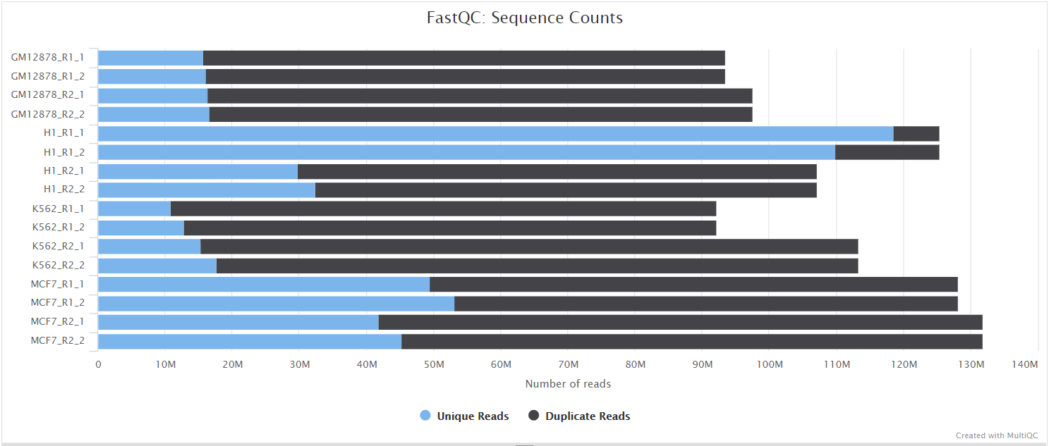
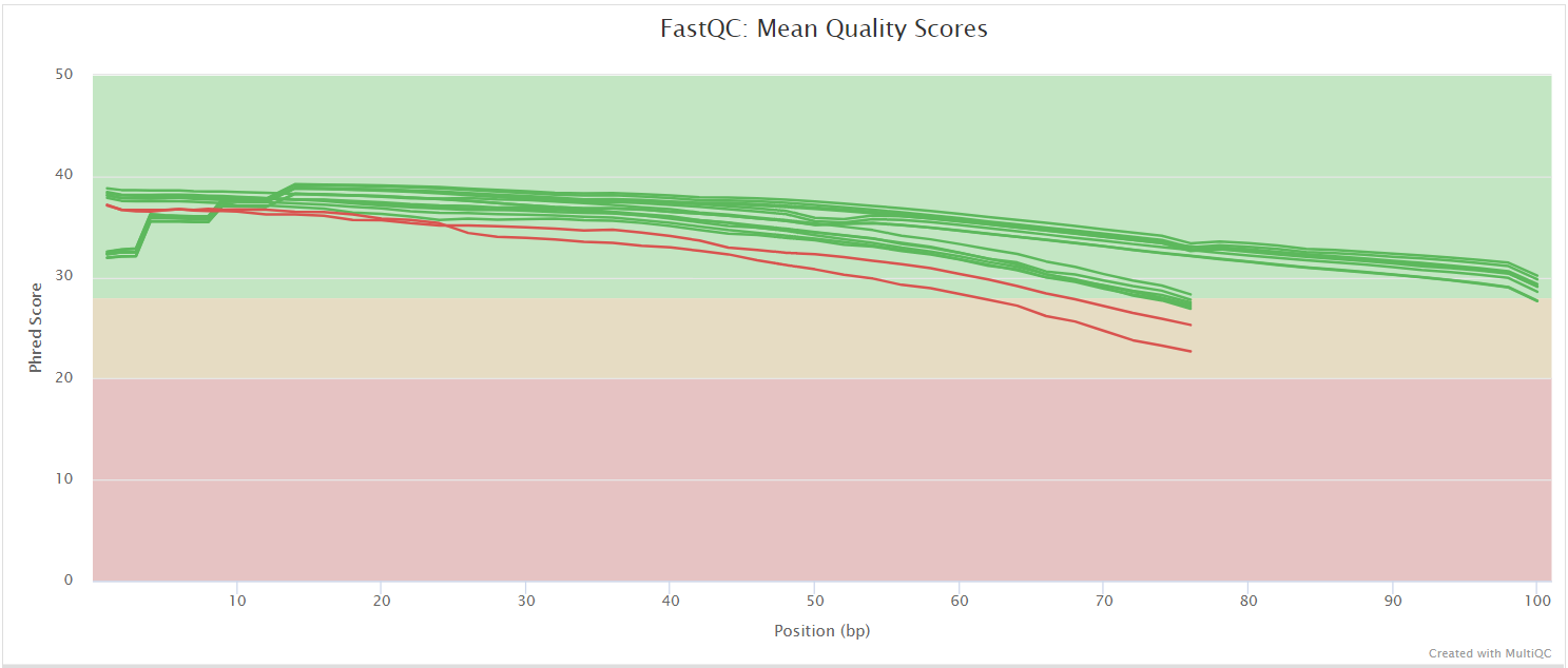
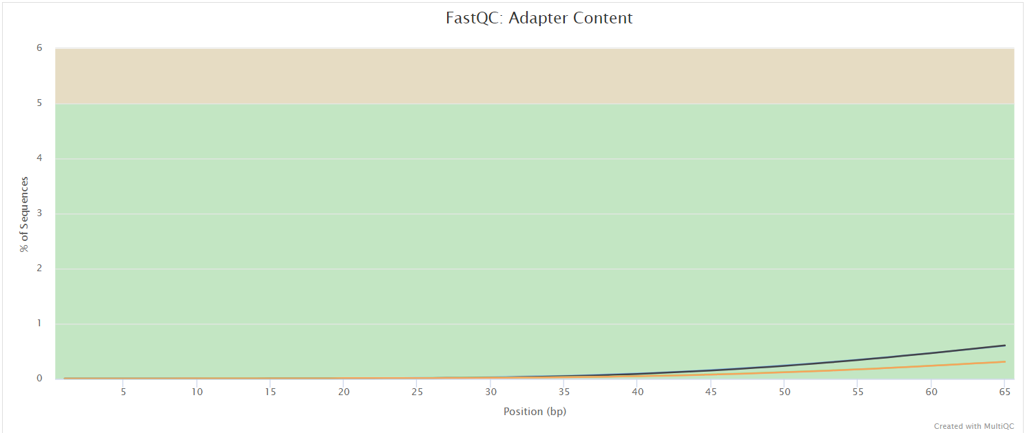
FastQC gives general quality metrics about your sequenced reads. It provides information about the quality score distribution across your reads, per base sequence content (%A/T/G/C), adapter contamination and overrepresented sequences. For further reading and documentation see the FastQC help pages.
UMI-tools extract
Output files
preprocessing/umitools/*.fastq.gz: If--save_umi_intermedsis specified, FastQ files after UMI extraction will be placed in this directory.*.log: Log file generated by the UMI-toolsextractcommand.
UMI-tools deduplicates reads based on unique molecular identifiers (UMIs) to address PCR-bias. Firstly, the UMI-tools extract command removes the UMI barcode information from the read sequence and adds it to the read name. Secondly, reads are deduplicated based on UMI identifier after mapping as highlighted in the UMI-tools dedup section.
To facilitate processing of input data which has the UMI barcode already embedded in the read name from the start, --skip_umi_extract can be specified in conjunction with --with_umi.
TrimGalore
Output files
preprocessing/trimgalore/*.fq.gz: If--save_trimmedis specified, FastQ files after adapter trimming will be placed in this directory.*_trimming_report.txt: Log file generated by Trim Galore!.
preprocessing/trimgalore/fastqc/*_fastqc.html: FastQC report containing quality metrics for read 1 (and read2 if paired-end) after adapter trimming.*_fastqc.zip: Zip archive containing the FastQC report, tab-delimited data file and plot images.
Trim Galore! is a wrapper tool around Cutadapt and FastQC to peform quality and adapter trimming on FastQ files. Trim Galore! will automatically detect and trim the appropriate adapter sequence. It is the default trimming tool used by this pipeline, however you can use fastp instead by specifying the --trimmer fastp parameter. You can specify additional options for Trim Galore! via the --extra_trimgalore_args parameters.
NB: TrimGalore! will only run using multiple cores if you are able to use more than > 5 and > 6 CPUs for single- and paired-end data, respectively. The total cores available to TrimGalore! will also be capped at 4 (7 and 8 CPUs in total for single- and paired-end data, respectively) because there is no longer a run-time benefit. See release notes and discussion whilst adding this logic to the nf-core/atacseq pipeline.
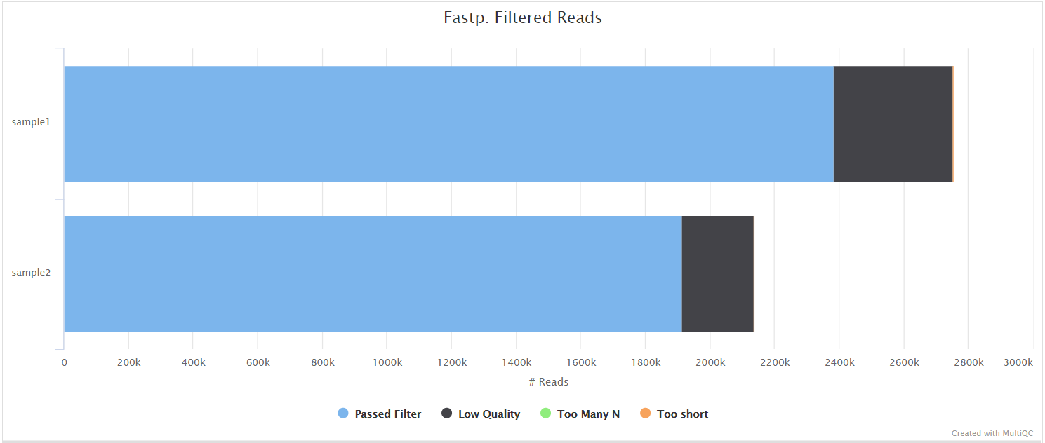
fastp
Output files
preprocessing/fastp/*.fastq.gz: If--save_trimmedis specified, FastQ files after adapter trimming will be placed in this directory.*.fastp.html: Trimming report in html format.*.fastp.json: Trimming report in json format.
preprocessing/fastp/log/*.fastp.log: Trimming log file.
preprocessing/fastp/fastqc/*_fastqc.html: FastQC report containing quality metrics for read 1 (and read2 if paired-end) after adapter trimming.*_fastqc.zip: Zip archive containing the FastQC report, tab-delimited data file and plot images.
fastp is a tool designed to provide fast, all-in-one preprocessing for FastQ files. It has been developed in C++ with multithreading support to achieve higher performance. fastp can be used in this pipeline for standard adapter trimming and quality filtering by setting the --trimmer fastp parameter. You can specify additional options for fastp via the --extra_fastp_args parameter.
BBSplit
Output files
preprocessing/bbsplit/*.fastq.gz: If--save_bbsplit_readsis specified FastQ files split by reference will be saved to the results directory. Reads from the main reference genome will be named “primary.fastq.gz”. Reads from contaminating genomes will be named “<SHORT_NAME>.fastq.gz” where<SHORT_NAME>is the first column in--bbsplit_fasta_listthat needs to be provided to initially build the index.*.txt: File containing statistics on how many reads were assigned to each reference.
BBSplit is a tool that bins reads by mapping to multiple references simultaneously, using BBMap. The reads go to the bin of the reference they map to best. There are also disambiguation options, such that reads that map to multiple references can be binned with all of them, none of them, one of them, or put in a special “ambiguous” file for each of them.
This functionality would be especially useful, for example, if you have mouse PDX samples that contain a mixture of human and mouse genomic DNA/RNA and you would like to filter out any mouse derived reads.
The BBSplit index will have to be built at least once with this pipeline by providing --bbsplit_fasta_list which has to be a file containing 2 columns: short name and full path to reference genome(s):
mm10,/path/to/mm10.faecoli,/path/to/ecoli.fasarscov2,/path/to/sarscov2.faYou can save the index by using the --save_reference parameter and then provide it via --bbsplit_index for future runs. As described in the Output files dropdown box above the FastQ files relative to the main reference genome will always be called *primary*.fastq.gz.
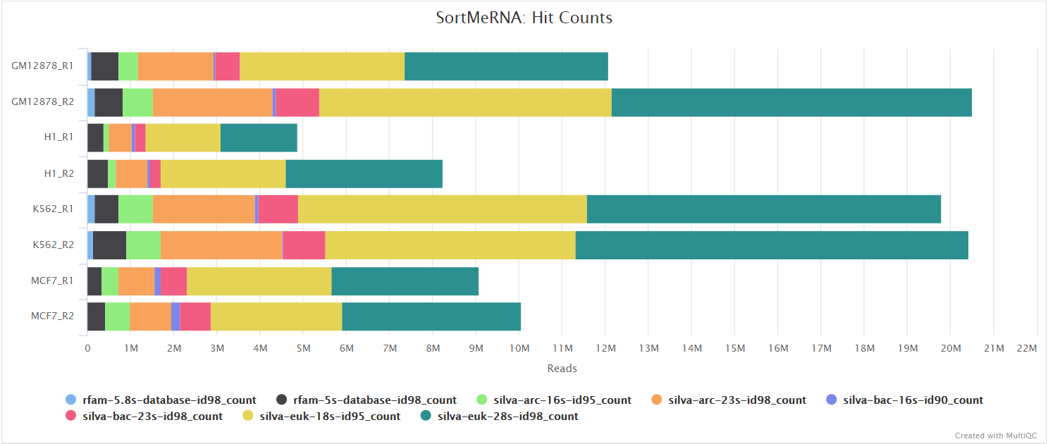
SortMeRNA
Output files
preprocessing/sortmerna/*.fastq.gz: If--save_non_ribo_readsis specified, FastQ files containing non-rRNA reads will be placed in this directory.*.log: Log file generated by SortMeRNA with information regarding reads that matched the reference database(s).
When --remove_ribo_rna is specified, the pipeline uses SortMeRNA for the removal of ribosomal RNA. By default, rRNA databases defined in the SortMeRNA GitHub repo are used. You can see an example in the pipeline Github repository in assets/rrna-default-dbs.txt which is used by default via the --ribo_database_manifest parameter. Please note that commercial/non-academic entities require licensing for SILVA for these default databases.
Alignment
STAR
Output files
alignment/star/original*.Aligned.out.bam: If--save_align_intermedsis specified the original BAM file containing read alignments to the reference genome will be placed in this directory.*.Aligned.toTranscriptome.out.bam: If--save_align_intermedsis specified the original BAM file containing read alignments to the transcriptome will be placed in this directory.
alignment/star/sorted*.genome.sorted.bam: Coordinate-sorted genome BAM file for each sample*.genome.sorted.bam.bai: Index for coordinate-sorted genome BAM file for each sample*.transcriptome.sorted.bam: Coordinate-sorted transcriptome BAM file for each sample*.transcriptome.sorted.bam.bai: Index for coordinate-sorted transcriptome BAM file for each sample
alignment/star/log/*.SJ.out.tab: File containing filtered splice junctions detected after mapping the reads.*.Log.final.out: STAR alignment report containing the mapping results summary.*.Log.outand*.Log.progress.out: STAR log files containing detailed information about the run. Typically only useful for debugging purposes.
alignment/star/unmapped/*.fastq.gz: If--save_unalignedis specified, FastQ files containing unmapped reads will be placed in this directory.
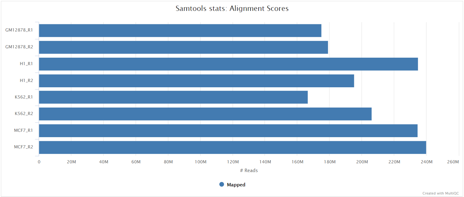
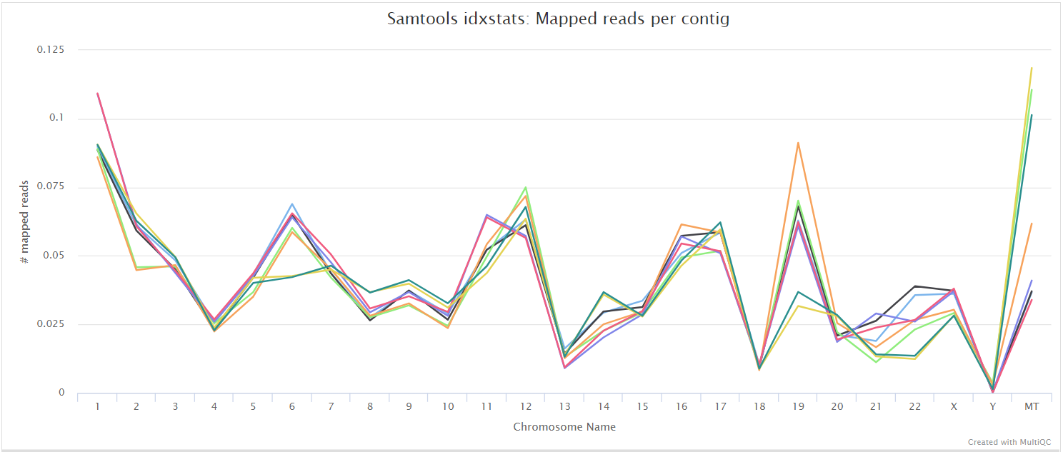
alignment/star/sorted/samtools_stats/- SAMtools
*.sorted.bam.flagstat,*.sorted.bam.idxstatsand*.sorted.bam.statsfiles generated from the sorted alignment files.
- SAMtools
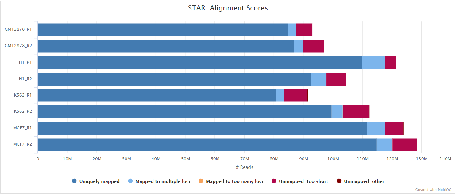
STAR is a read aligner designed for splice aware mapping typical of RNA sequencing data. STAR stands for Spliced Transcripts Alignment to a Reference, and has been shown to have high accuracy and outperforms other aligners by more than a factor of 50 in mapping speed, but it is memory intensive. Using --aligner star_salmon is the default alignment and quantification option.
The STAR section of the MultiQC report shows a bar plot with alignment rates: good samples should have most reads as Uniquely mapped and few Unmapped reads.
The original BAM files generated by the selected alignment algorithm are further processed with SAMtools to sort them by coordinate, for indexing, as well as to generate read mapping statistics.
UMI-tools deduplication
Output files
<ALIGNER>/<SAMPLE>.umi_dedup.sorted.bam: If--save_umi_intermedsis specified the UMI deduplicated, coordinate sorted BAM file containing read alignments will be placed in this directory.<SAMPLE>.umi_dedup.sorted.bam.bai: If--save_umi_intermedsis specified the BAI index file for the UMI deduplicated, coordinate sorted BAM file will be placed in this directory.<SAMPLE>.umi_dedup.sorted.bam.csi: If--save_umi_intermeds --bam_csi_indexis specified the CSI index file for the UMI deduplicated, coordinate sorted BAM file will be placed in this directory.
<ALIGNER>/umitools/*_edit_distance.tsv: Reports the (binned) average edit distance between the UMIs at each position.*_per_umi.tsv: UMI-level summary statistics.*_per_umi_per_position.tsv: Tabulates the counts for unique combinations of UMI and position.
The content of the files above is explained in more detail in the UMI-tools documentation.
After extracting the UMI information from the read sequence (see UMI-tools extract), the second step in the removal of UMI barcodes involves deduplicating the reads based on both mapping and UMI barcode information using the UMI-tools dedup command. This will generate a filtered BAM file after the removal of PCR duplicates.
Riboseq-specific QC
Read distribution metrics around annotated protein coding regions or based on alignments alone, plus related metrics.
Ribo-TISH quality
Output files
riboseq_qc/ribotish/*_qual.txt: text-format data on read distribution around annotated protein coding regions on user provided transcripts*_qual.pdf: PDF-format representation of read distribution around annotated protein coding regions on user provided transcripts*.para.py: P-site offsets for different reads lengths in python code dict format
Ribotricer detect-orfs QC outputs
Output files
riboseq_qc/ribotricer/*_read_length_dist.pdf: PDF-format read length distribution as quality control*_metagene_plots.pdf: Metagene plots for quality control*_protocol.txt: txt file containing inferred protocol if it was inferred (not supplied as input)*_metagene_profiles_5p.tsv: Metagene profile aligning with the start codon*_metagene_profiles_3p.tsv: Metagene profile aligning with the stop codon
ORF predictions
Ribo-TISH predict
Output files
orf_predictions/ribotish/*_pred.txtthresholded ORF predictions from Ribo-TISH*_all.txtunthresholded ORF predictions from Ribo-TISH*_transprofile.pyRPF P-site profile for each transcript from Ribo-TISH
orf_predictions/ribotish_all/allsamples_pred.txtthresholded ORF predictions from Ribo-TISH ran over all samples at onceallsamples_all.txtunthresholded ORF predictions from Ribo-TISH ran over all samples at onceallsamples_transprofile.pyRPF P-site profile for each transcript from Ribo-TISH ran over all samples at once
Ribotricer detect-orfs
Output files
orf_predictions/ribotricer/*_translating_ORFs.tsvTSV with ORFs assessed as translating in the assocciated BAM file*_psite_offsets.txt: If the P-site offsets are not provided, txt file containing the derived relative offsets.
Quantification
Quantification is done by passing transcriptome-level alignment BAM files to Salmon, producing the following outputs:
Output files
quantification/tx2gene.tsv: Tab-delimited file containing gene to transcripts ids mappings.
quantification/salmon/- salmon.merged.gene_counts.tsv`: Matrix of gene-level raw counts across all samples.
- salmon.merged.gene_tpm.tsv`: Matrix of gene-level TPM values across all samples.
- salmon.merged.gene.rds
: RDS object that can be loaded in R that contains a [SummarizedExperiment](https://bioconductor.org/packages/release/bioc/html/SummarizedExperiment.html) container with the TPM (abundance), estimated counts (counts) and transcript length (length`) in the assays slot for genes. - salmon.merged.gene_counts_scaled.tsv`: Matrix of gene-level library size-scaled counts across all samples.
- salmon.merged.gene__scaled.rds
: RDS object that can be loaded in R that contains a [SummarizedExperiment](https://bioconductor.org/packages/release/bioc/html/SummarizedExperiment.html) container with the TPM (abundance), estimated library size-scaled counts (counts) and transcript length (length`) in the assays slot for genes. - salmon.merged.gene_counts_length_scaled.tsv`: Matrix of gene-level length-scaled counts across all samples.
- salmon.merged.gene_length_scaled.rds
: RDS object that can be loaded in R that contains a [SummarizedExperiment](https://bioconductor.org/packages/release/bioc/html/SummarizedExperiment.html) container with the TPM (abundance), estimated length-scaled counts (counts) and transcript length (length`) in the assays slot for genes. - salmon.merged.transcript_counts.tsv`: Matrix of isoform-level raw counts across all samples.
- salmon.merged.transcript_tpm.tsv`: Matrix of isoform-level TPM values across all samples.
- salmon.merged.transcript.rds
: RDS object that can be loaded in R that contains a [SummarizedExperiment](https://bioconductor.org/packages/release/bioc/html/SummarizedExperiment.html) container with the TPM (abundance), estimated isoform-level raw counts (counts) and transcript length (length`) in the assays slot for transcripts.
Raw outputs from Salmon are available for each sample:
Output files
quantification/salmon/<SAMPLE>/aux_info/: Auxiliary info e.g. versions and number of mapped reads.cmd_info.json: Information about the Salmon quantification command, version and options.lib_format_counts.json: Number of fragments assigned, unassigned and incompatible.libParams/: Contains the fileflenDist.txtfor the fragment length distribution.logs/: Contains the filesalmon_quant.loggiving a record of Salmon’s quantification.quant.genes.sf: Salmon gene-level quantification of the sample, including feature length, effective length, TPM, and number of reads.quant.sf: Salmon transcript-level quantification of the sample, including feature length, effective length, TPM, and number of reads.
Translational efficiency
anota2seq produces the following outputs:
Output files
translational_efficiency/anota2seq*.total_mRNA.anota2seq.results.tsv: anota2seq results for the ‘total mRNA’ analysis, describing differences in RNA levels across conditions for RNA-seq samples. See https://rdrr.io/bioc/anota2seq/man/anota2seqGetOutput.html for description of output columns.*.translated_mRNA.anota2seq.results.tsv: anota2seq results for the ‘translated mRNA’ analysis, describing differences in RNA levels across conditions for Ribo-seq samples. See https://rdrr.io/bioc/anota2seq/man/anota2seqGetOutput.html for description of output columns.*.mRNA_abundance.anota2seq.results.tsv: anota2seq results for the ‘mRNA abunance’ analysis, describing changes across conditions consistent between total mRNA and translated RNA (RNA-seq and Riboseq samples). See https://rdrr.io/bioc/anota2seq/man/anota2seqGetOutput.html for description of output columns.*.buffering.anota2seq.results.tsv: anota2seq results for the ‘buffering’ analysis, describing stable levels of translated RNA (from riboseq samples) across conditions, despite changes in total mRNA. See https://rdrr.io/bioc/anota2seq/man/anota2seqGetOutput.html for description of output columns.*.translation.anota2seq.results.tsv: anota2seq results for the ‘translation’ analysis, describing differences in translation across conditions, being differences in translated RNA levels not explained by total RNA levels. See https://rdrr.io/bioc/anota2seq/man/anota2seqGetOutput.html for description of output columns.*.fold_change.png: A fold change plot in PNG format, from anota2seq’s anota2seqPlotFC() method.*.interaction_p_distribution.pdf: The distribution of p-values and adjusted p-values for the omnibus interaction (both using densities and histograms). The second page of the pdf displays the same plots but for the RVM statistics if RVM is used.*.residual_distribution_summary.jpeg: Summary plot for assessing normal distribution of regression residuals.*.residual_vs_fitted.jpeg: QC plot showing residuals against fitted values.*.rvm_fit_for_all_contrasts_group.jpg: QC plot showing the CDF of variance (theoretical vs empirical), all contrasts.*.rvm_fit_for_interactions.jpg: QC plot showing the CDF of variance (theoretical vs empirical), for interactions.*.rvm_fit_for_omnibus_group.jpg: QC plot showing the CDF of variance (theoretical vs empirical), for omnibus group.*.simulated_vs_obt_dfbetas_without_interaction.pdf: Bar graphs of the frequencies of outlier dfbetas using different dfbetas thresholds..Anota2seqDataSet.rds: Serialised Anota2seqDataSet object*.R_sessionInfo.log: dump of R SessionInfo
A key plot is the fold change plot produced by anota2seq:
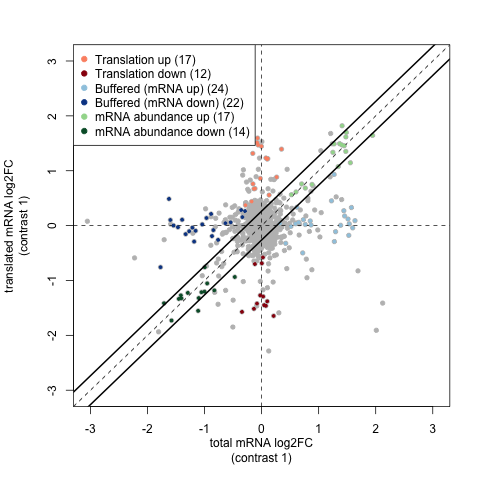
By plotting fold changes for RNA-seq and Ribo-seq data against one another this shows the relative importance of buffering, translation changes etc in these samples.
MultiQC
Output files
multiqc/multiqc_report.html: a standalone HTML file that can be viewed in your web browser.multiqc_data/: directory containing parsed statistics from the different tools used in the pipeline.
MultiQC is a visualization tool that generates a single HTML report summarising all samples in your project. Most of the pipeline QC results are visualised in the report and further statistics are available in the report data directory.
Results generated by MultiQC collate pipeline QC from supported tools i.e. FastQC, Cutadapt, SortMeRNA, STAR, RSEM, HISAT2, Salmon, SAMtools, Picard, RSeQC, Qualimap, Preseq and featureCounts. Additionally, various custom content has been added to the report to assess the output of dupRadar, DESeq2 and featureCounts biotypes, and to highlight samples failing a mimimum mapping threshold or those that failed to match the strand-specificity provided in the input samplesheet. The pipeline has special steps which also allow the software versions to be reported in the MultiQC output for future traceability. For more information about how to use MultiQC reports, see http://multiqc.info.
Workflow reporting and genomes
Reference genome files
Output files
genome/*.fa,*.gtf,*.gff,*.bed,.tsv: If the--save_referenceparameter is provided then all of the genome reference files will be placed in this directory.
genome/index/star/: Directory containing STAR indices.hisat2/: Directory containing HISAT2 indices.
A number of genome-specific files are generated by the pipeline because they are required for the downstream processing of the results. If the --save_reference parameter is provided then these will be saved in the genome/ directory. It is recommended to use the --save_reference parameter if you are using the pipeline to build new indices so that you can save them somewhere locally. The index building step can be quite a time-consuming process and it permits their reuse for future runs of the pipeline to save disk space.
Pipeline information
Output files
pipeline_info/- Reports generated by Nextflow:
execution_report.html,execution_timeline.html,execution_trace.txtandpipeline_dag.dot/pipeline_dag.svg. - Reports generated by the pipeline:
pipeline_report.html,pipeline_report.txtandsoftware_versions.yml. Thepipeline_report*files will only be present if the--email/--email_on_failparameter’s are used when running the pipeline. - Reformatted samplesheet files used as input to the pipeline:
samplesheet.valid.csv. - Parameters used by the pipeline run:
params.json.
- Reports generated by Nextflow:
Nextflow provides excellent functionality for generating various reports relevant to the running and execution of the pipeline. This will allow you to troubleshoot errors with the running of the pipeline, and also provide you with other information such as launch commands, run times and resource usage.