Output

This document describes the output produced by the pipeline. Most of the plots are taken from the MultiQC report, which summarises results at the end of the pipeline.

Pipeline overview

The pipeline is built using Nextflow
and processes data using the following steps:

* nf-core/bacass: Output
* Pipeline overview
* Quality trimming and QC
* Short Read Trimming
* Short Read RAW QC
* Long Read Trimming
* Long Read RAW QC
* Taxonomic classification
* Kraken2 report screenshot
* Assembly Output
* Assembly Visualization with Bandage
* Assembly QC with QUAST
* Annotation with Prokka
* Report

Quality trimming and QC

Short Read Trimming

This step quality trims the end of reads, removes degenerate or too short reads and if needed,
combines reads coming from multiple sequencing runs.

*Output directory: {sample_id}/trimming/shortreads/*

* \*.fastq.gz
* trimmed (and combined reads)

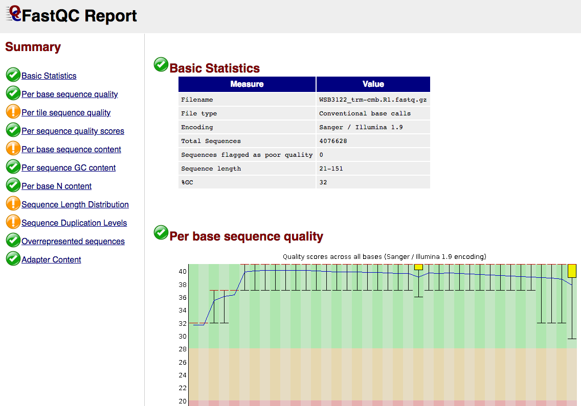
Short Read RAW QC

This step runs FastQC which produces
general quality metrics on your (trimmed) samples and plots them.

*Output directory: {sample_id}/trimming/shortreads/*

* \*_fastqc.html
* FastQC report, containing quality metrics for your trimmed reads
* \*_fastqc.zip
* zip file containing the FastQC report, tab-delimited data file and plot images

For further reading and documentation see the FastQC help.

Long Read Trimming

This step performs long read trimming on Nanopore input (if provided).

*Output directory: {sample_id}/trimming/longreads/*

* trimmed.fastq
* The trimmed FASTQ file

Long Read RAW QC

These steps perform long read QC for input data (if provided).

*Output directory: {sample_id}/QC_Longreads/*

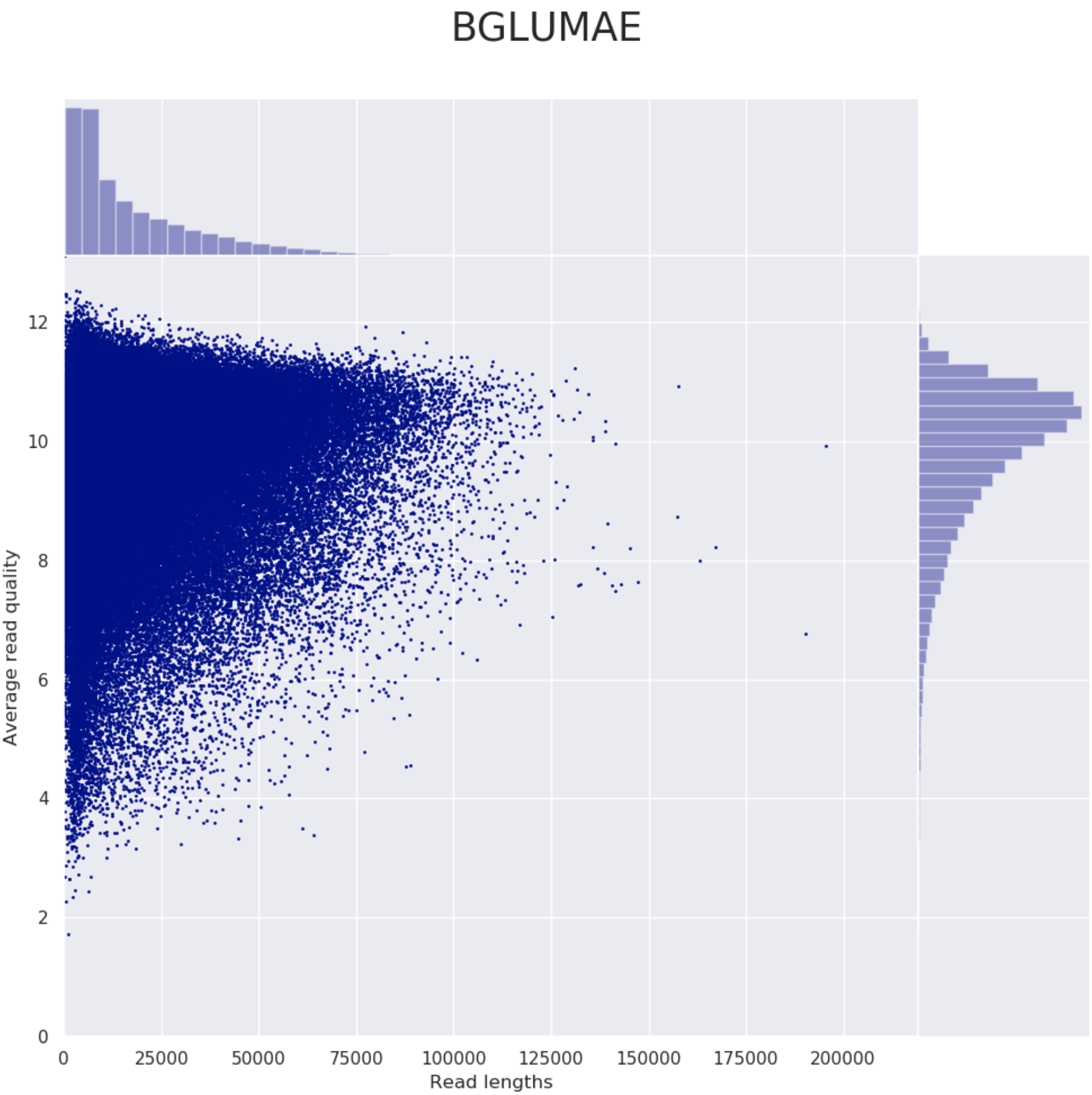
* NanoPlot
* PycoQC

Please refer to the documentation of NanoPlot and PycoQC if you want to know more about the plots created by these tools.

Example plot from Nanoplot:

Taxonomic classification

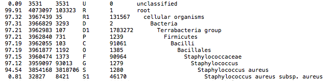
This QC step classifies your reads using Kraken2 a k-mer based approach. This helps to identify samples that have purity
issues. Ideally you will not want to assemble reads from samples that are contaminated or contain
multiple species. If you like to visualize the report, try
Pavian or Krakey.

*Output directory: {sample}/*

* \*_kraken2.report
* Classification in the Kraken(1) report format. See
webpage for more details

Kraken2 report screenshot

Assembly Output

Trimmed reads are assembled with Unicycler in short or hybrid assembly modes. For long-read assembly, there are also canu and miniasm available.
Unicycler is a pipeline on its own, which at least for Illumina reads mainly acts as a frontend to Spades with added polishing steps.

*Output directory: {sample_id}/unicycler*

* {sample}_assembly.fasta
* Final assembly
* {sample}_assembly.gfa
* Final assembly in Graphical Fragment Assembly (GFA) format
* {sample}_unicycler.log
* Log file summarizing steps and intermediate results on the Unicycler execution

Check out the Unicycler documentation for more information on Unicycler output.

*Output directory: {sample_id}/canu*

Check out the Canu documentation for more information on Canu output.

*Output directory: {sample_id}/miniasm*

* consensus
* The consensus sequence created by miniasm

Check out the Miniasm documentation for more information on Miniasm output.

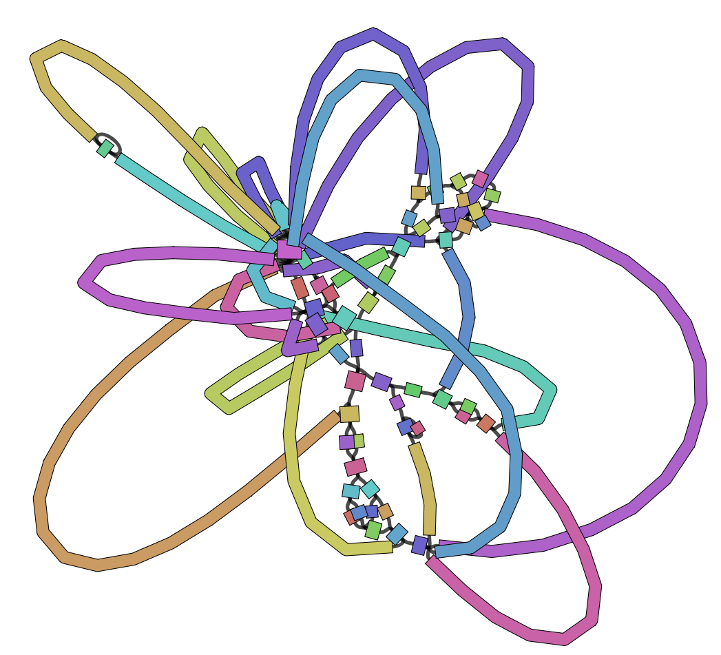
Assembly Visualization with Bandage

The GFA file produced in the assembly step with Unicycler can be used to visualise the assembly graph, which is
done here with Bandage. We highly recommend to run the Bandage GUI for more versatile visualisation options (annotations etc).

*Output directory: {sample_id}/unicycler*

* {sample}_assembly.png
* Bandage visualization of assembly

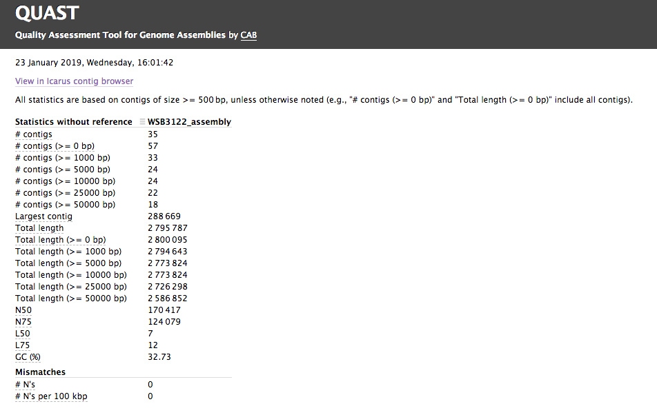
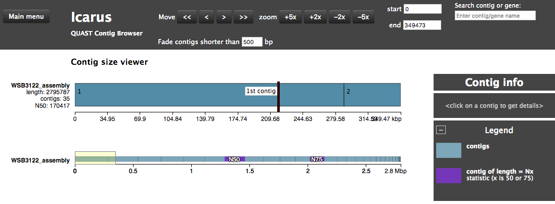
Assembly QC with QUAST

The assembly QC is performed with QUAST.
It reports multiple metrics including number of contigs, N50, lengths etc in form of an html report.
It further creates an HTML file with integrated contig viewer (Icarus).

*Output directory: {sample_id}/QUAST*

* icarus.html
* QUAST's contig browser as HTML
* report.html
* QUAST assembly QC as HTML report

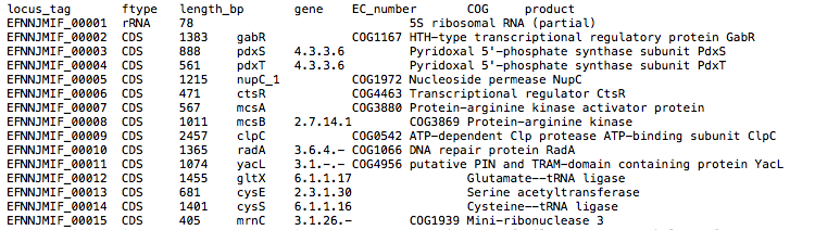
Annotation with Prokka

The assembly is annotated with Prokka which acts as frontend
for several annotation tools and includes rRNA and ORF predictions. See its documentation for a full description of all output files.

*Output directory: {sample_id}/{sample_id}_annotation*

Report

Some pipeline results are visualised by MultiQC, which is a visualisation tool that generates a single HTML report summarising all samples in your project. Further statistics are available in within the report data directory.

The pipeline has special steps which allow the software versions used to be reported in the MultiQC output for future traceability.

*Output directory: results/multiqc*

* Project_multiqc_report.html
* MultiQC report - a standalone HTML file that can be viewed in your web browser
* Project_multiqc_data/
* Directory containing parsed statistics from the different tools used in the pipeline

For more information about how to use MultiQC reports, see http://multiqc.info