nf-core/eager
A fully reproducible and state-of-the-art ancient DNA analysis pipeline
2.2.1). The latest stable release is2.5.3.22.10.6.Learn more.Introduction
Running the pipeline
Quick Start
Before you start you should change into the output directory you wish your results to go in. This will guarantee, that when you start the Nextflow job, it will place all the log files and ‘working’ folders in the corresponding output directory, (and not wherever else you may have executed the run from)
The typical command for running the pipeline is as follows:
nextflow run nf-core/eager --input '*_R{1,2}.fastq.gz' --fasta 'some.fasta' -profile standard,dockerwhere the reads are from FASTQ files of the same pairing.
This will launch the pipeline with the docker configuration profile. See below
for more information about profiles.
Note that the pipeline will create the following files in your working directory:
work # Directory containing the Nextflow working filesresults # Finished results (configurable, see below).nextflow.log # Log file from Nextflow # Other Nextflow hidden files, eg. history of pipeline runs and old logs.To see the the nf-core/eager pipeline help message run: nextflow run nf-core/eager --help
If you want to configure your pipeline interactively using a graphical user
interface, please visit nf-co.re
launch. Select the eager pipeline and
the version you intend to run, and follow the on-screen instructions to create a
config for your pipeline run.
Updating the pipeline
When you run the above command, Nextflow automatically pulls the pipeline code from GitHub and stores it as a cached version. When running the pipeline after this, it will always use the cached version if available - even if the pipeline has been updated since. To make sure that you’re running the latest version of the pipeline, make sure that you regularly update the cached version of the pipeline:
nextflow pull nf-core/eagerReproducibility
It’s a good idea to specify a pipeline version when running the pipeline on your data. This ensures that a specific version of the pipeline code and software are used when you run your pipeline. If you keep using the same tag, you’ll be running the same version of the pipeline, even if there have been changes to the code since.
First, go to the nf-core/eager releases
page and find the latest version
number - numeric only (eg. 2.2.0). Then specify this when running the pipeline
with -r (one hyphen) - eg. -r 2.2.0.
This version number will be logged in reports when you run the pipeline, so that you’ll know what you used when you look back in the future.
Additionally, nf-core/eager pipeline releases are named after Swabian German Cities. The first release V2.0 is named “Kaufbeuren”. Future releases are named after cities named in the Swabian league of Cities.
Automatic Resubmission
By default, if a pipeline step fails, nf-core/eager will resubmit the job with twice the amount of CPU and memory. This will occur two times before failing.
Core Nextflow arguments
NB: These options are part of Nextflow and use a single hyphen (pipeline parameters use a double-hyphen).
-profile
Use this parameter to choose a configuration profile. Profiles can give configuration presets for different compute environments.
Several generic profiles are bundled with the pipeline which instruct the pipeline to use software packaged using different methods (Docker, Singularity, Conda) - see below.
We highly recommend the use of Docker or Singularity containers for full pipeline reproducibility, however when this is not possible, Conda is also supported.
The pipeline also dynamically loads configurations from https://github.com/nf-core/configs when it runs, making multiple config profiles for various institutional clusters available at run time. For more information and to see if your system is available in these configs please see the nf-core/configs documentation.
Note that multiple profiles can be loaded, for example: -profile test,docker -
the order of arguments is important! They are loaded in sequence, so later
profiles can overwrite earlier profiles.
If -profile is not specified, the pipeline will run locally and expect all
software to be installed and available on the PATH. This is not recommended.
Important: If running nf-core/eager on a cluster - ask your system administrator what profile to use.
docker- A generic configuration profile to be used with Docker
- Pulls software from Docker Hub:
nfcore/eager
singularity- A generic configuration profile to be used with Singularity
- Pulls software from Docker Hub:
nfcore/eager
condatest- A profile with a complete configuration for automated testing
- Includes links to test data so needs no other parameters
Institution Specific Profiles These are profiles specific to certain HPC clusters, and are centrally maintained at nf-core/configs. Those listed below are regular users of nf-core/eager, if you don’t see your own institution here check the nf-core/configs repository.
uzh- A profile for the University of Zurich Research Cloud
- Loads Singularity and defines appropriate resources for running the pipeline.
binac- A profile for the BinAC cluster at the University of Tuebingen 0 Loads Singularity and defines appropriate resources for running the pipeline
shh- A profile for the S/CDAG cluster at the Department of Archaeogenetics of the Max Planck Institute for the Science of Human History
- Loads Singularity and defines appropriate resources for running the pipeline
Pipeline Specific Institution Profiles There are also pipeline-specific institution profiles. I.e., we can also offer a profile which sets special resource settings to specific steps of the pipeline, which may not apply to all pipelines. This can be seen at nf-core/configs under conf/pipelines/eager/.
We currently offer a nf-core/eager specific profile for
shh- A profiler for the S/CDAG cluster at the Department of Archaeogenetics of the Max Planck Institute for the Science of Human History
- In addition to the nf-core wide profile, this also sets the MALT resources to match our commonly used databases
Further institutions can be added at nf-core/configs. Please ask the eager developers to add your institution to the list above, if you add one!
-resume
Specify this when restarting a pipeline. Nextflow will used cached results from any pipeline steps where the inputs are the same, continuing from where it got to previously.
You can also supply a run name to resume a specific run: -resume [run-name].
Use the nextflow log command to show previous run names.
-c
Specify the path to a specific config file (this is a core Nextflow command). See the nf-core website documentation for more information.
Custom resource requests
Each step in the pipeline has a default set of requirements for number of CPUs,
memory and time. For most of the steps in the pipeline, if the job exits with an
error code of 143 (exceeded requested resources) it will automatically
resubmit with higher requests (2 x original, then 3 x original). If it still
fails after three times then the pipeline is stopped.
Whilst these default requirements will hopefully work for most people with most
data, you may find that you want to customise the compute resources that the
pipeline requests. You can do this by creating a custom config file. For
example, to give the workflow process star 32GB of memory, you could use the
following config:
process { withName: bwa { memory = 32.GB }}See the main Nextflow documentation for more information.
If you are likely to be running nf-core pipelines regularly it may be a good
idea to request that your custom config file is uploaded to the
nf-core/configs git repository. Before you do this please can you test that
the config file works with your pipeline of choice using the -c parameter (see
definition below). You can then create a pull request to the nf-core/configs
repository with the addition of your config file, associated documentation file
(see examples in
nf-core/configs/docs),
and amending
nfcore_custom.config
to include your custom profile.
If you have any questions or issues please send us a message on
Slack on the #configs
channel.
-name
Name for the pipeline run. If not specified, Nextflow will automatically generate a random mnemonic.
This is used in the MultiQC report (if not default) and in the summary HTML / e-mail (always).
NB: Single hyphen (core Nextflow option)
Running in the background
Nextflow handles job submissions and supervises the running jobs. The Nextflow process must run until the pipeline is finished.
Nextflow handles job submissions on SLURM or other environments, and supervises
running the jobs. Thus the Nextflow process must run until the pipeline is
finished. We recommend that you put the process running in the background
through screen / tmux or similar tool. Alternatively you can run Nextflow
within a cluster job submitted your job scheduler.
To create a screen session:
screen -R nf-core/eagerTo disconnect, press ctrl+a then d.
To reconnect, type:
screen -r nf-core/eagerto end the screen session while in it type exit.
Alternatively, the Nextflow -bg flag launches Nextflow in the background,
detached from your terminal so that the workflow does not stop if you log out of
your session. The logs are saved to a file.
Nextflow memory requirements
In some cases, the Nextflow Java virtual machines can start to request a large
amount of memory. We recommend adding the following line to your environment to
limit this (typically in ~/.bashrc or ~./bash_profile):
NXF_OPTS='-Xms1g -Xmx4g'Pipeline Options
Input
--input
There are two possible ways of supplying input sequencing data to nf-core/eager. The most efficient but more simplistic is supplying direct paths (with wildcards) to your FASTQ or BAM files, with each file or pair being considered a single library and each one run independently. TSV input requires creation of an extra file by the user and extra metadata, but allows more powerful lane and library merging.
Direct Input Method
This method is where you specify with --input, the path locations of FASTQ
(optionally gzipped) or BAM file(s). This option is mutually exclusive to the
TSV input method, which is used for more complex input
configurations such as lane and library merging.
When using the direct method of --input you can specify one or multiple
samples in one or more directories files. File names must be unique, even if
in different directories.
By default, the pipeline assumes you have paired-end data. If you want to run
single-end data you must specify --single_end
For example, for a single set of FASTQs, or multiple paired-end FASTQ files in one directory, you can specify:
--input 'path/to/data/sample_*_{1,2}.fastq.gz'If you have multiple files in different directories, you can use additional
wildcards (*) e.g.:
--input 'path/to/data/*/sample_*_{1,2}.fastq.gz'⚠️ It is not possible to run a mixture of single-end and paired-end files in one run with the paths
--inputmethod! Please see the TSV input method for possibilities.
Please note the following requirements:
- Valid file extensions:
.fastq.gz,.fastq,.fq.gz,.fq,.bam. - The path must be enclosed in quotes
- The path must have at least one
*wildcard character - When using the pipeline with paired end data, the path must use
{1,2}notation to specify read pairs. - Files names must be unique, having files with the same name, but in different
directories is not sufficient
- This can happen when a library has been sequenced across two sequencers on the same lane. Either rename the file, try a symlink with a unique name, or merge the two FASTQ files prior input.
- Due to limitations of downstream tools (e.g. FastQC), sample IDs may be
truncated after the first
.in the name, Ensure file names are unique prior to this! - For input BAM files you should provide a small decoy reference genome with
pre-made indices, e.g. the human mtDNA or phiX genome, for the mandatory
parameter
--fastain order to avoid long computational time for generating the index files of the reference genome, even if you do not actual need a reference genome for any downstream analyses.
TSV Input Method
Alternatively to the direct input method, you can supply
to --input a path to a TSV file that contains paths to FASTQ/BAM files and
additional metadata. This allows for more complex procedures such as merging of
sequencing data across lanes, sequencing runs, sequencing configuration types,
and samples.
The use of the TSV --input method is recommended when performing
more complex procedures such as lane or library merging. You do not need to
specify --single_end, --bam, --colour_chemistry, -udg_type etc. when
using TSV input - this is defined within the TSV file itself. You can only
supply a single TSV per run (i.e. --input '*.tsv' will not work).
This TSV should look like the following:
| Sample_Name | Library_ID | Lane | Colour_Chemistry | SeqType | Organism | Strandedness | UDG_Treatment | R1 | R2 | BAM |
|---|---|---|---|---|---|---|---|---|---|---|
| JK2782 | JK2782 | 1 | 4 | PE | Mammoth | double | full | https://github.com/nf-core/test-datasets/raw/eager/testdata/Mammoth/fastq/JK2782_TGGCCGATCAACGA_L008_R1_001.fastq.gz.tengrand.fq.gz | https://github.com/nf-core/test-datasets/raw/eager/testdata/Mammoth/fastq/JK2782_TGGCCGATCAACGA_L008_R2_001.fastq.gz.tengrand.fq.gz | NA |
| JK2802 | JK2802 | 2 | 2 | SE | Mammoth | double | full | https://github.com/nf-core/test-datasets/raw/eager/testdata/Mammoth/fastq/JK2802_AGAATAACCTACCA_L008_R1_001.fastq.gz.tengrand.fq.gz | https://github.com/nf-core/test-datasets/raw/eager/testdata/Mammoth/fastq/JK2802_AGAATAACCTACCA_L008_R2_001.fastq.gz.tengrand.fq.gz | NA |
A template can be taken from here.
⚠️ Cells must not contain spaces before or after strings, as this will make the TSV unreadable by Nextflow. Strings containing spaces should be wrapped in quotes.
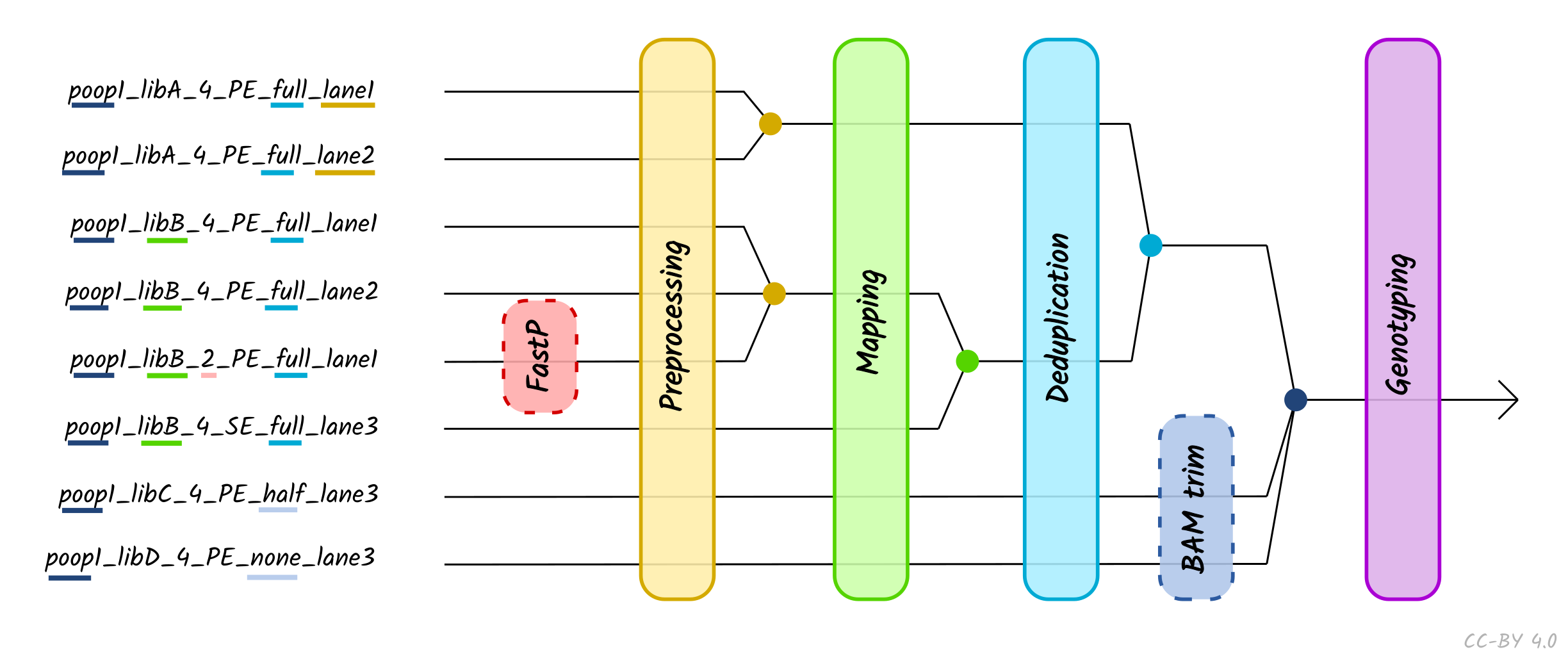
When using TSV_input, nf-core/eager will merge FASTQ files of libraries with the
same Library_ID but different Lanes values after adapter clipping (and
merging), assuming all other metadata columns are the same. If you have the same
Library_ID but with different SeqType, this will be merged directly after
mapping prior BAM filtering. Finally, it will also merge BAM files with the same
Sample_ID but different Library_ID after duplicate removal, but prior to
genotyping. Please see caveats to this below.
Column descriptions are as follows:
- Sample_Name: A text string containing the name of a given sample of which there can be multiple libraries. All libraries with the same sample name and same SeqType will be merged after deduplication.
- Library_ID: A text string containing a given library, which there can be multiple sequencing lanes (with the same SeqType).
- Lane: A number indicating which lane the library was sequenced on. Files from the libraries sequenced on different lanes (and different SeqType) will be concatenated after read clipping and merging.
- Colour Chemistry A number indicating whether the Illumina sequencer the library was sequenced on was a 2 (e.g. Next/NovaSeq) or 4 (Hi/MiSeq) colour chemistry machine. This informs whether poly-G trimming (if turned on) should be performed.
- SeqType: A text string of either ‘PE’ or ‘SE’, specifying paired end (with both an R1 [or forward] and R2 [or reverse]) and single end data (only R1 [forward], or BAM). This will affect lane merging if different per library.
- Organism: A text string of the organism name of the sample or ‘NA’. This currently has no functionality and can be set to ‘NA’, but will affect lane/library merging if different per library
- Strandedness: A text string indicating whether the library type is ‘single’ or ‘double’. This will affect lane/library merging if different per library.
- UDG_Treatment: A text string indicating whether the library was generated with UDG treatment - either ‘full’, ‘half’ or ‘none’. Will affect lane/library merging if different per library.
- R1: A text string of a file path pointing to a forward or R1 FASTQ file. This can be used with the R2 column. File names must be unique, even if they are in different directories.
- R2: A text string of a file path pointing to a reverse or R2 FASTQ file, or ‘NA’ when single end data. This can be used with the R1 column. File names must be unique, even if they are in different directories.
- BAM: A text string of a file path pointing to a BAM file, or ‘NA’. Cannot be specified at the same time as R1 or R2, both of which should be set to ‘NA’
For example, the following TSV table:
| Sample_Name | Library_ID | Lane | Colour_Chemistry | SeqType | Organism | Strandedness | UDG_Treatment | R1 | R2 | BAM |
|---|---|---|---|---|---|---|---|---|---|---|
| JK2782 | JK2782 | 7 | 4 | PE | Mammoth | double | full | data/JK2782_TGGCCGATCAACGA_L007_R1_001.fastq.gz.tengrand.fq.gz | data/JK2782_TGGCCGATCAACGA_L007_R2_001.fastq.gz.tengrand.fq.gz | NA |
| JK2782 | JK2782 | 8 | 4 | PE | Mammoth | double | full | data/JK2782_TGGCCGATCAACGA_L008_R1_001.fastq.gz.tengrand.fq.gz | data/JK2782_TGGCCGATCAACGA_L008_R2_001.fastq.gz.tengrand.fq.gz | NA |
| JK2802 | JK2802 | 7 | 4 | PE | Mammoth | double | full | data/JK2802_AGAATAACCTACCA_L007_R1_001.fastq.gz.tengrand.fq.gz | data/JK2802_AGAATAACCTACCA_L007_R2_001.fastq.gz.tengrand.fq.gz | NA |
| JK2802 | JK2802 | 8 | 4 | SE | Mammoth | double | full | data/JK2802_AGAATAACCTACCA_L008_R1_001.fastq.gz.tengrand.fq.gz | NA | NA |
will have the following effects:
- After AdapterRemoval, and prior to mapping, FASTQ files from lane 7 and lane 8
with the same
SeqType(and all other metadata columns) will be concatenated together for each Library. - After mapping, and prior BAM filtering, BAM files with the same with different
SeqType(but with all other metadata columns the same) will be merged together for each Library. - After duplicate removal, BAM files with
Library_IDs with the sameSample_Nameand the sameUDG_Treatmentwill be merged together. - If BAM trimming is turned on, all post-trimming BAMs (i.e. non-UDG and
half-UDG ) will be merged with UDG-treated (untreated) BAMs, if they have the
same
Sample_Name.
Note the following important points and limitations for setting up:
- The TSV must use actual tabs (not spaces) between cells.
- File names must be unique regardless of file path, due to risk of
over-writing (see:
https://github.com/nextflow-io/nextflow/issues/470).
- If it is ‘too late’ and you already have duplicate file names, a workaround is to concatenate the FASTQ files together and supply this to a nf-core/eager run. The only downside is that you will not get independent FASTQC results for each file.
- Lane IDs must be unique for each sequencing of each library.
- If you have a library sequenced e.g. on Lane 8 of two HiSeq runs, you can give a fake lane ID (e.g. 20) for one of the FASTQs, and the libraries will still be processed correctly.
- This also applies to the SeqType column, i.e. with the example above, if one run is PE and one run is SE, you need to give fake lane IDs to one of the runs as well.
- All BAM files must be specified as
SEunderSeqType.- You should provide a small decoy reference genome with pre-made indices, e.g.
the human mtDNA or phiX genome, for the mandatory parameter
--fastain order to avoid long computational time for generating the index files of the reference genome, even if you do not actual need a reference genome for any downstream analyses.
- You should provide a small decoy reference genome with pre-made indices, e.g.
the human mtDNA or phiX genome, for the mandatory parameter
- nf-core/eager will only merge multiple lanes of sequencing runs with the same single-end or paired-end configuration
- Accordingly nf-core/eager will not merge lanes of FASTQs with BAM files
(unless you use
--run_convertbam), as only FASTQ files are lane-merged together. - Same libraries that are sequenced on different sequencing configurations (i.e
single- and paired-end data), will be merged after mapping and will always
be considered ‘paired-end’ during downstream processes
- Important running DeDup in this context is not recommended, as PE and SE data at the same position will not be evaluated as duplicates. Therefore not all duplicates will be removed.
- When you wish to run PE/SE data together
-dedupper markduplicatesis therefore preferred. - An error will be thrown if you try to merge both PE and SE and also supply
--skip_merging. - If you truly want to mix SE data and PE data but using mate-pair info for PE mapping, please run FASTQ preprocessing mapping manually and supply BAM files for downstream processing by nf-core/eager
- If you regularly want to run the situation above, please leave a feature request on github.
- DamageProfiler, NuclearContamination, MTtoNucRatio and PreSeq are performed on each unique library separately after deduplication (but prior same-treated library merging).
- nf-core/eager functionality such as
--run_trim_bamwill be applied to only non-UDG (UDG_Treatment: none) or half-UDG (UDG_Treatment: half) libraries. - Qualimap is run on each sample, after merging of libraries (i.e. your values will reflect the values of all libraries combined - after being damage trimmed etc.).
- Genotyping will be typically performed on each
sampleindependently, as normally all libraries will have been merged together. However, if you have a mixture of single-stranded and double-stranded libraries, you will normally need to genotype separately. In this case you must give each the SS and DS libraries distinctSample_IDs; otherwise you will receive afile collisionerror in steps such assexdeterrmine, and then you will need to merge these yourself. We will consider changing this behaviour in the future if there is enough interest.
--udg_type
Defines whether Uracil-DNA glycosylase (UDG) treatment was used to remove DNA damage on the sequencing libraries.
Specify 'none' if no treatment was performed. If you have partial UDG treated
data (Rohland et al 2016), specify
'half'. If you have complete UDG treated data (Briggs et al.
2010), specify 'full'.
When also using PMDtools specifying 'half' will use a different model for DNA
damage assessment in PMDTools (PMDtools: --UDGhalf). Specify 'full' and the
PMDtools DNA damage assessment will use CpG context only (PMDtools: --CpG).
Default: 'none'.
Tip: You should provide a small decoy reference genome with pre-made indices, e.g. the human mtDNA genome, for the mandatory parameter
--fastain order to avoid long computational time for generating the index files of the reference genome, even if you do not actual need a reference genome for any downstream analyses.
--single_stranded
Indicates libraries are single stranded.
Currently only affects MALTExtract, where it will switch on damage patterns
calculation mode to single-stranded, (MaltExtract: --singleStranded) and
genotyping with pileupCaller where a different method is used (pileupCaller:
--singleStrandMode). Default: false.
Only required when using the ‘Path’ method of --input.
--single_end
Indicates libraries were sequenced with single-end sequencing chemistries (i.e. only a R1 file is present). If not supplied, input data assumed to be paired-end by default.
Only required when using the ‘Path’ method of --input.
--colour_chemistry
Specifies which Illumina colour chemistry a library was sequenced with. This
informs whether to perform poly-G trimming (if --complexity_filter_poly_g is
also supplied). Only 2 colour chemistry sequencers (e.g. NextSeq or NovaSeq) can
generate uncertain poly-G tails (due to ‘G’ being indicated via a no-colour
detection). Default is ‘4’ to indicate e.g. HiSeq or MiSeq platforms, which do
not require poly-G trimming. Options: 2, 4. Default: 4
Only required when using the ‘Path’ method of --input.
--bam
Specifies the input file type to --input is in BAM format. This will
automatically also apply --single_end.
Only required when using the ‘Path’ method of --input.
Input Data Additional Options
--snpcapture_bed
Can be used to set a path to a BED file (3/6 column format) of SNP positions of a reference genome, to calculate SNP captured libraries on-target efficiency. This should be used for array or in-solution SNP capture protocols such as 390K, 1240K, etc. If supplied, on-target metrics are automatically generated for you by qualimap.
--run_convertinputbam
Allows you to convert an input BAM file back to FASTQ for downstream processing. Note this is required if you need to perform AdapterRemoval and/or polyG clipping.
If not turned on, BAMs will automatically be sent to post-mapping steps.
Reference Genomes
All nf-core/eager runs require a reference genome in FASTA format to map reads against to.
In addition we provide various options for indexing of different types of reference genomes (based on the tools used in the pipeline). nf-core/eager can index reference genomes for you (with options to save these for other analysis), but you can also supply your pre-made indices.
Supplying pre-made indices saves time in pipeline execution and is especially advised when running multiple times on the same cluster system, for example. You can even add a resource specific profile that sets paths to pre-computed reference genomes, saving time when specifying these.
⚠️ you must always supply a reference file. If you want to use functionality that does not require one, supply a small decoy genome such as phiX or the human mtDNA genome.
--fasta
You specify the full path to your reference genome here. The FASTA file can have
any file suffix, such as .fasta, .fna, .fa, .FastA etc. You may also
supply a gzipped reference files, which will be unzipped automatically for you.
For example:
--fasta '/<path>/<to>/my_reference.fasta'You need to provide an input FASTA even if you do not do any mapping (e.g.
supplying BAM files). You should use a small decoy reference genome with pre-made
indices, e.g. the human mtDNA genome, for the mandatory parameter --fasta in
order to avoid long computational time for generating the index files of the
reference genome.
If you don’t specify appropriate
--bwa_index,--fasta_indexparameters (see below), the pipeline will create these indices for you automatically. Note that you can save the indices created for you for later by giving the--save_referenceflag. You must select either a--fastaor--genome
--genome (using iGenomes)
Alternatively, the pipeline config files come bundled with paths to the Illumina iGenomes reference index files. If running with Docker or AWS, the configuration is set up to use the AWS-iGenomes resource.
There are 31 different species supported in the iGenomes references. To run the
pipeline, you must specify which to use with the --genome flag.
You can find the keys to specify the genomes in the iGenomes config file under
conf/ on the nf-core/eager GitHub
repository. Common genomes that are supported
are:
- Human
--genome GRCh37--genome GRCh38
- Mouse *
--genome GRCm38
- Drosophila *
--genome BDGP6
- S. cerevisiae *
--genome 'R64-1-1'
* Not bundled with nf-core eager by default.
Note that you can use the same configuration set-up to save sets of reference files for your own use, even if they are not part of the iGenomes resource. See the Nextflow documentation for instructions on where to save such a file.
The syntax for this reference configuration is as follows:
params { genomes { 'GRCh37' { fasta = '<path to the iGenomes genome fasta file>' } // Any number of additional genomes, key is used with --genome }}You must select either a
--fastaor--genome
--bwa_index
If you want to use pre-existing bwa index indices, please supply the
directory to the FASTA you also specified in --fasta (see above).
nf-core/eager will automagically detect the index files by searching for the
FASTA filename with the corresponding bwa index file suffixes.
⚠️ pre-built indices must currently be built on non-gzipped FASTA files due to limitations of
samtools. However once indices have been built, you can re-gzip the FASTA file as nf-core will unzip this particular file for you.
For example:
nextflow run nf-core/eager \-profile test,docker \--input '*{R1,R2}*.fq.gz'--fasta 'results/reference_genome/bwa_index/BWAIndex/Mammoth_MT_Krause.fasta' \--bwa_index 'results/reference_genome/bwa_index/BWAIndex/'
bwa indexdoes not give you an option to supply alternative suffixes/names for these indices. Thus, the file names generated by this command must not be changed, otherwise nf-core/eager will not be able to find them.
--bt2_index
If you want to use pre-existing bt2 index indices, please supply the
directory to the FASTA you also specified in --fasta (see above).
nf-core/eager will automagically detect the index files by searching for the
FASTA filename with the corresponding bt2 index file suffixes.
⚠️ pre-built indices must currently be built on non-gzipped FASTA files due to limitations of
samtools. However once indices have been built, you can re-gzip the FASTA file as nf-core will unzip this particular file for you.
For example:
nextflow run nf-core/eager \-profile test,docker \--input '*{R1,R2}*.fq.gz'--fasta 'results/reference_genome/bwa_index/BWAIndex/Mammoth_MT_Krause.fasta' \--bwa_index 'results/reference_genome/bt2_index/BT2Index/'
bowtie2-builddoes not give you an option to supply alternative suffixes/names for these indices. Thus, the file names generated by this command must not be changed, otherwise nf-core/eager will not be able to find them.
--fasta_index
If you want to use a pre-existing samtools faidx index, use this to specify
the required FASTA index file for the selected reference genome. This should be
generated by samtools faidx and has a file suffix of .fai
For example:
--fasta_index 'Mammoth_MT_Krause.fasta.fai'--seq_dict
If you want to use a pre-existing picard CreateSequenceDictionary dictionary
file, use this to specify the required .dict file for the selected reference
genome.
⚠️ pre-built indices must currently be built on non-gzipped FASTA files due to limitations of
samtools. However once indices have been built, you can re-gzip the FASTA file as nf-core will unzip this particular file for you.
For example:
--seq_dict 'Mammoth_MT_Krause.dict'--large_ref
This parameter is required to be set for large reference genomes. If your
reference genome is larger than 3.5GB, the samtools index calls in the
pipeline need to generate CSI indices instead of BAI indices to compensate
for the size of the reference genome (with samtools: -c). This parameter is
not required for smaller references (including the human hg19 or
grch37/grch38 references), but >4GB genomes have been shown to need CSI
indices. Default: off
modifies SAMtools index command:
-c
--save_reference
Use this if you do not have pre-made reference FASTA indices for bwa,
samtools and picard. If you turn this on, the indices nf-core/eager
generates for you and will be saved in the
<your_output_dir>/results/reference_genomes for you. If not supplied,
nf-core/eager generated index references will be deleted.
Output
--outdir
The output directory where the results will be saved.
-w / -work-dir
The output directory where intermediate files will be saved. It is highly
recommended that this is the same path as --outdir, otherwise you may ‘lose’
your intermediate files if you need to re-run a pipeline. By default, if this
flag is not given, the intermediate files will be saved in a work/ and
.nextflow/ directory from wherever you have run nf-core/eager from.
--publish_dir_mode
Nextflow mode for ‘publishing’ final results files i.e. how to move final files
into your --outdir from working directories. Options: ‘symlink’, ‘rellink’,
‘link’, ‘copy’, ‘copyNoFollow’, ‘move’. Default: ‘copy’.
It is recommended to select
copy(default) if you plan to regularly delete intermediate files fromwork/.
Other run specific parameters
--max_memory
Use to set a top-limit for the default memory requirement for each process.
Should be a string in the format integer-unit. eg. --max_memory '8.GB'. If not
specified, will be taken from the configuration in the -profile flag.
--max_time
Use to set a top-limit for the default time requirement for each process. Should
be a string in the format integer-unit. eg. --max_time '2.h'. If not
specified, will be taken from the configuration in the -profile flag.
--max_cpus
When not using a institute specific -profile, you can use this parameter to
set a top-limit for the default CPU requirement for each process. This is
not the maximum number of CPUs that can be used for the whole pipeline, but the
maximum number of CPUs each program can use for each program submission (known
as a process).
Do not set this higher than what is available on your workstation or computing
node can provide. If you’re unsure, ask your local IT administrator for details
on compute node capabilities! Should be a string in the format integer-unit. eg.
--max_cpus 1. If not specified, will be taken from the configuration in the
-profile flag.
--email
Set this parameter to your e-mail address to get a summary e-mail with details
of the run sent to you when the workflow exits. If set in your user config file
(~/.nextflow/config) then you don’t need to specify this on the command line
for every run.
Note that this functionality requires either mail or sendmail to be
installed on your system.
--email_on_fail
Set this parameter to your e-mail address to get a summary e-mail with details
of the run if it fails. Normally would be the same as in --email. If set in
your user config file (~/.nextflow/config) then you don’t need to specify this
on the command line for every run.
Note that this functionality requires either
sendmailto be installed on your system.
--plaintext_email
Set to receive plain-text e-mails instead of HTML formatted.
--monochrome_logs
Set to disable colourful command line output and live life in monochrome.
--multiqc_config
Specify a path to a custom MultiQC configuration file.
--custom_config_version
Provide git commit id for custom Institutional configs hosted at
nf-core/configs. This was implemented for reproducibility purposes. Default is
set to master.
\#\# Download and use config file with following git commit id--custom_config_version d52db660777c4bf36546ddb188ec530c3ada1b96Step skipping parameters
Some of the steps in the pipeline can be executed optionally. If you specify specific steps to be skipped, there won’t be any output related to these modules.
--skip_fastqc
Turns off FastQC pre- and post-Adapter Removal, to speed up the pipeline. Use of this flag is most common when data has been previously pre-processed and the post-Adapter Removal mapped reads are being re-mapped to a new reference genome.
--skip_adapterremoval
Turns off adapter trimming and paired-end read merging. Equivalent to setting
both --skip_collapse and --skip_trim.
--skip_preseq
Turns off the computation of library complexity estimation.
--skip_deduplication
Turns off duplicate removal methods DeDup and MarkDuplicates respectively. No duplicates will be removed on any data in the pipeline.
--skip_damage_calculation
Turns off the DamageProfiler module to compute DNA damage profiles.
--skip_qualimap
Turns off QualiMap and thus does not compute coverage and other mapping metrics.
Complexity Filtering Options
More details can be seen in the fastp documentation
If using TSV input, this is performed per lane separately.
--complexity_filter_poly_g
Performs a poly-G tail removal step in the beginning of the pipeline using
fastp, if turned on. This can be useful for trimming ploy-G tails from
short-fragments sequenced on two-colour Illumina chemistry such as NextSeqs
(where no-fluorescence is read as a G on two-colour chemistry), which can
inflate reported GC content values.
--complexity_filter_poly_g_min
This option can be used to define the minimum length of a poly-G tail to begin
low complexity trimming. By default, this is set to a value of 10 unless the
user has chosen something specifically using this option.
Modifies fastp parameter:
--poly_g_min_len
Adapter Clipping and Merging Options
These options handle various parts of adapter clipping and read merging steps.
More details can be seen in the AdapterRemoval documentation
If using TSV input, this is performed per lane separately.
⚠️
--skip_trimwill skip adapter clipping AND quality trimming (n, base quality). It is currently not possible skip one or the other.
--clip_forward_adaptor
Defines the adapter sequence to be used for the forward read. By default, this
is set to 'AGATCGGAAGAGCACACGTCTGAACTCCAGTCAC'.
Modifies AdapterRemoval parameter:
--adapter1
--clip_reverse_adaptor
Defines the adapter sequence to be used for the reverse read in paired end
sequencing projects. This is set to 'AGATCGGAAGAGCGTCGTGTAGGGAAAGAGTGTA' by
default.
Modifies AdapterRemoval parameter:
--adapter2
--clip_readlength
Defines the minimum read length that is required for reads after merging to be
considered for downstream analysis after read merging. Default is 30.
Note that performing read length filtering at this step is not reliable for
correct endogenous DNA calculation, when you have a large percentage of very
short reads in your library - such as retrieved in single-stranded library
protocols. When you have very few reads passing this length filter, it will
artificially inflate your endogenous DNA by creating a very small denominator.
In these cases it is recommended to set this to 0, and use
--bam_filter_minreadlength instead, to filter out ‘un-usable’ short reads
after mapping.
Modifies AdapterRemoval parameter:
--minlength
--clip_min_read_quality
Defines the minimum read quality per base that is required for a base to be
kept. Individual bases at the ends of reads falling below this threshold will be
clipped off. Default is set to 20.
Modifies AdapterRemoval parameter:
--minquality
--clip_min_adap_overlap
Sets the minimum overlap between two reads when read merging is performed.
Default is set to 1 base overlap.
Modifies AdapterRemoval parameter:
--minadapteroverlap
--skip_collapse
Turns off the paired-end read merging.
For example
--skip_collapse --input '*_{R1,R2}_*.fastq'It is important to use the paired-end wildcard globbing, as --skip_collapse
can only be used on paired-end data!
⚠️ If you provide this option together with --clip_readlength set to
something (as is by default), you may end up removing single reads from either
the pair1 or pair2 file. These will be NOT be mapped when aligning with either
bwa or bowtie, as both can only accept one (forward) or two (forward and
reverse) FASTQs as input.
Modifies AdapterRemoval parameter:
--collapse
--skip_trim
Turns off adapter AND quality trimming.
For example:
--skip_trim --input '*.fastq'⚠️ it is not possible to keep quality trimming (n or base quality) on, and skip adapter trimming.
⚠️ it is not possible to turn off one or the other of quality
trimming or n trimming. i.e. –trimns –trimqualities are both given
or neither. However setting quality in --clip_min_read_quality to 0 would
theoretically turn off base quality trimming.
Modifies AdapterRemoval parameters:
--trimns --trimqualities --adapter1 --adapter2
--preserve5p
Turns off quality based trimming at the 5p end of reads when any of the –trimns, –trimqualities, or –trimwindows options are used. Only 3p end of reads will be removed.
This also entirely disables quality based trimming of collapsed reads, since both ends of these are informative for PCR duplicate filtering. Described here.
Modifies AdapterRemoval parameters:
--preserve5p
--mergedonly
Specify that only merged reads are sent downstream for analysis.
Singletons (i.e. reads missing a pair), or un-merged reads (where there wasn’t sufficient overlap) are discarded.
You may want to use this if you want ensure only the best quality reads for your
analysis, but with the penalty of potentially losing still valid data (even if
some reads have slightly lower quality). It is highly recommended when using
--dedupper 'dedup' (see below).
Read Mapping Parameters
If using TSV input, mapping is performed at the library level, i.e. after lane merging.
--mapper
Specify which mapping tool to use. Options are BWA aln ('bwaaln'), BWA mem
('bwamem'), circularmapper ('circularmapper'), or bowtie2 (bowtie2). BWA
aln is the default and highly suited for short-read ancient DNA. BWA mem can be
quite useful for modern DNA, but is rarely used in projects for ancient DNA.
CircularMapper enhances the mapping procedure to circular references, using the
BWA algorithm but utilizing a extend-remap procedure (see Peltzer et al 2016,
Genome Biology for details). Bowtie2 is similar to BWA aln, and has recently
been suggested to provide slightly better results under certain conditions
(Poullet and Orlando 2020), as well
as providing extra functionality (such as FASTQ trimming). Default is ‘bwaaln’
More documentation can be seen for each tool under:
BWA (default)
These parameters configure mapping algorithm parameters.
--bwaalnn
Defines how many mismatches from the reference are allowed in a read. By default
set to 0.04 (following recommendations of Schubert et al. (2012 BMC
Genomics)), if you’re uncertain what
to set check out this Shiny App
for more information on how to set this parameter efficiently.
Modifies bwa aln parameter:
-n
--bwaalnk
Modifies the number of mismatches in the seed during the seeding phase in the
bwa aln mapping algorithm. Default is set to 2.
Modifies BWA aln parameter:
-k
--bwaalnl
Configures the length of the seed used during seeding. Default is set to be
‘turned off’ at the recommendation of Schubert et al. (2012 BMC
Genomics) for ancient DNA with
1024.
Note: Despite being recommended, turning off seeding can result in long runtimes!
Modifies BWA aln parameter:
-l
CircularMapper
--circularextension
The number of bases to extend the reference genome with. By default this is set
to 500 if not specified otherwise.
Modifies circulargenerator and realignsamfile parameter:
-e
--circulartarget
The chromosome in your FASTA reference that you’d like to be treated as
circular. By default this is set to MT but can be configured to match any
other chromosome.
Modifies circulargenerator parameter:
-s
--circularfilter
If you want to filter out reads that don’t map to a circular chromosome, turn this on. By default this option is turned off.
Bowtie2
--bt2_alignmode
The type of read alignment to use. Options are ‘local’ or ‘end-to-end’. Local allows only partial alignment of read, with ends of reads possibly ‘soft-clipped’ (i.e. remain unaligned/ignored), if the soft-clipped alignment provides best alignment score. End-to-end requires all nucleotides to be aligned. Default is ‘local’, following Cahill et al (2018) and Poullet and Orlando 2020.
Modifies Bowtie2 parameters:
--very-fast --fast --sensitive --very-sensitive --very-fast-local --fast-local --sensitive-local --very-sensitive-local
--bt2_sensitivity
The Bowtie2 ‘preset’ to use. Options: ‘no-preset’ ‘very-fast’, ‘fast’,
‘sensitive’, or ‘very-sensitive’. These strings apply to both --bt2_alignmode
options. See the Bowtie2
manual
for actual settings. Default is ‘sensitive’ (following Poullet and Orlando
(2020), when running damaged-data
without UDG treatment)
Modifies Bowtie2 parameters:
--very-fast --fast --sensitive --very-sensitive --very-fast-local --fast-local --sensitive-local --very-sensitive-local
--bt2n
The number of mismatches allowed in the seed during seed-and-extend procedure of
Bowtie2. This will override any values set with --bt2_sensitivity. Can either
be 0 or 1. Default: 0 (i.e. use--bt2_sensitivity defaults).
Modifies Bowtie2 parameters:
-N
--bt2l
The length of the seed sub-string to use during seeding. This will override any
values set with --bt2_sensitivity. Default: 0 (i.e. use--bt2_sensitivity
defaults: 20 for local and 22 for
end-to-end.
Modifies Bowtie2 parameters:
-L
-bt2_trim5
Number of bases to trim at the 5’ (left) end of read prior alignment. Maybe useful when left-over sequencing artefacts of in-line barcodes present Default: 0
Modifies Bowtie2 parameters:
-bt2_trim5
-bt2_trim3
Number of bases to trim at the 3’ (right) end of read prior alignment. Maybe useful when left-over sequencing artefacts of in-line barcodes present Default: 0.
Modifies Bowtie2 parameters:
-bt2_trim3
Removal of Host-Mapped Reads
These parameters are used for removing mapped reads from the original input FASTQ files, usually in the context of uploading the original FASTQ files to a public read archive (NCBI SRA/EBI ENA/DDBJ SRA).
These flags will produce FASTQ files almost identical to your input files, except that reads with the same read ID as one found in the mapped bam file, are either removed or ‘masked’ (every base replaced with Ns).
This functionality allows you to provide other researchers who wish to re-use your data to apply their own adapter removal/read merging procedures, while maintaining anonymity for sample donors - for example with microbiome research.
If using TSV input, mapped read removal is performed per library, i.e. after lane merging.
--hostremoval_input_fastq
Create pre-Adapter Removal FASTQ files without reads that mapped to reference (e.g. for public upload of privacy sensitive non-host data)
--hostremoval_mode
Read removal mode. Completely remove mapped reads from the file(s) ('remove')
or just replace mapped reads sequence by N ('replace')
Modifies extract_map_reads.py parameter:
-m
Read Filtering and Conversion Parameters
Users can configure to keep/discard/extract certain groups of reads efficiently in the nf-core/eager pipeline.
If using TSV input, filtering is performed library, i.e. after lane merging.
This module utilises samtools view and filter_bam_fragment_length.py
--run_bam_filtering
Turns on the bam filtering module for either mapping quality filtering or unmapped read treatment.
⚠️ this is required for metagenomic screening!
--bam_mapping_quality_threshold
Specify a mapping quality threshold for mapped reads to be kept for downstream
analysis. By default keeps all reads and is therefore set to 0 (basically
doesn’t filter anything).
Modifies samtools view parameter:
-q
--bam_filter_minreadlength
Specify minimum length of mapped reads. This filtering will apply at the same time as mapping quality filtering.
If used instead of minimum length read filtering at AdapterRemoval, this can be useful to get more realistic endogenous DNA percentages, when most of your reads are very short (e.g. in single-stranded libraries) and would otherwise be discarded by AdapterRemoval (thus making an artificially small denominator for a typical endogenous DNA calculation). Note in this context you should not perform mapping quality filtering nor discarding of unmapped reads to ensure a correct denominator of all reads, for the endogenous DNA calculation.
Modifies filter_bam_fragment_length.py parameter:
-l
--bam_unmapped_type
Defines how to proceed with unmapped reads: 'discard' removes all unmapped
reads, keep keeps both unmapped and mapped reads in the same BAM file, 'bam'
keeps unmapped reads as BAM file, 'fastq' keeps unmapped reads as FastQ file,
both keeps both BAM and FASTQ files. Default is discard. keep is what
would happen if --run_bam_filtering was not supplied.
Note that in all cases, if --bam_mapping_quality_threshold is also supplied,
mapping quality filtering will still occur on the mapped reads.
⚠️ --bam_unmapped_type 'fastq' is required for metagenomic
screening!
Modifies samtools view parameter:
-f4 -F4
Read DeDuplication Parameters
If using TSV input, deduplication is performed per library, i.e. after lane merging.
--dedupper
Sets the duplicate read removal tool. By default uses markduplicates from
Picard. Alternatively an ancient DNA specific read deduplication tool dedup
(Peltzer et al. 2016) is offered.
This utilises both ends of paired-end data to remove duplicates (i.e. true exact duplicates, as markduplicates will over-zealously deduplicate anything with the same starting position even if the ends are different). DeDup should only be used solely on paired-end data otherwise suboptimal deduplication can occur if applied to either single-end or a mix of single-end/paired-end data.
Note that if you run without the --mergedonly flag for AdapterRemoval, DeDup
will likely fail. If you absolutely want to use both PE and SE data, you can
supply the --dedup_all_merged flag to consider singletons to also be merged
paired-end reads. This may result in over-zealous deduplication.
--dedup_all_merged
Sets DeDup to treat all reads as merged reads. This is useful if reads are for
example not prefixed with M_ in all cases. Therefore, this can be used as a
workaround when also using a mixture of paired-end and single-end data, however
this is not recommended (see above).
Modifies dedup parameter:
-m
Library Complexity Estimation Parameters
nf-core/eager uses Preseq on mapped reads as one method to calculate library
complexity. If DeDup is used, Preseq uses the histogram output of DeDup,
otherwise the sorted non-duplicated BAM file is supplied. Furthermore, if
paired-end read collapsing is not performed, the -P flag is used.
--preseq_step_size
Can be used to configure the step size of Preseq’s c_curve method. Can be
useful when only few and thus shallow sequencing results are used for
extrapolation.
Modifies preseq c_curve parameter:
-s
DNA Damage Assessment Parameters
More documentation can be seen in the follow links for:
If using TSV input, DamageProfiler is performed per library, i.e. after lane merging. PMDtools and BAM Trimming is run after library merging of same-named library BAMs that have the same type of UDG treatment. BAM Trimming is only performed on non-UDG and half-UDG treated data.
--damageprofiler_length
Specifies the length filter for DamageProfiler. By default set to 100.
Modifies DamageProfile parameter:
-l
--damageprofiler_threshold
Specifies the length of the read start and end to be considered for profile
generation in DamageProfiler. By default set to 15 bases.
Modifies DamageProfile parameter:
-t
--damageprofiler_yaxis
Specifies what the maximum misincorporation frequency should be displayed as, in
the DamageProfiler damage plot. This is set to 0.30 (i.e. 30%) by default as
this matches the popular mapDamage2.0
program. However, the default behaviour of DamageProfiler is to ‘autoscale’ the
y-axis maximum to zoom in on any possible damage that may occur (e.g. if the
damage is about 10%, the highest value on the y-axis would be set to 0.12). This
‘autoscale’ behaviour can be turned on by specifying the number to 0. Default:
0.30.
Modifies DamageProfile parameter:
-yaxis_damageplot
--run_pmdtools
Specifies to run PMDTools for damage based read filtering and assessment of DNA damage in sequencing libraries. By default turned off.
--pmdtools_range
Specifies the range in which to consider DNA damage from the ends of reads. By
default set to 10.
Modifies PMDTools parameter:
--range
--pmdtools_threshold
Specifies the PMDScore threshold to use in the pipeline when filtering BAM files
for DNA damage. Only reads which surpass this damage score are considered for
downstream DNA analysis. By default set to 3 if not set specifically by the
user.
Modifies PMDTools parameter:
--threshold
--pmdtools_reference_mask
Can be used to set a path to a reference genome mask for PMDTools.
--pmdtools_max_reads
The maximum number of reads used for damage assessment in PMDtools. Can be used to significantly reduce the amount of time required for damage assessment in PMDTools. Note that a too low value can also obtain incorrect results.
Modifies PMDTools parameter:
-n
Feature Annotation Statistics
If you’re interested in looking at coverage stats for certain features on your reference such as genes, SNPs etc., you can use the following bedtools module for this purpose.
More documentation on bedtools can be seen in the bedtools documentation
If using TSV input, bedtools is run after library merging of same-named library BAMs that have the same type of UDG treatment.
--run_bedtools_coverage
Specifies to turn on the bedtools module, producing statistics for breadth (or percent coverage), and depth (or X fold) coverages.
--anno_file
Specify the path to a GFF/BED containing the feature coordinates (or any
acceptable input for bedtools coverage).
Must be in quotes.
BAM Trimming Parameters
For some library preparation protocols, users might want to clip off damaged
bases before applying genotyping methods. This can be done in nf-core/eager
automatically by turning on the --run_trim_bam parameter.
More documentation can be seen in the bamUtil documentation
--run_trim_bam
Turns on the BAM trimming method. Trims off [n] bases from reads in the
deduplicated BAM file. Damage assessment in PMDTools or DamageProfiler remains
untouched, as data is routed through this independently. BAM trimming is
typically performed to reduce errors during genotyping that can be caused by
aDNA damage.
BAM trimming will only be performed on libraries indicated as --udg_type 'none' or --udg_type 'half'. Complete UDG treatment (‘full’) should have
removed all damage. The amount of bases that will be trimmed off can be set
separately for libraries with --udg_type 'none' and 'half' (see
--bamutils_clip_half_udg_left / --bamutils_clip_half_udg_right /
--bamutils_clip_none_udg_left / --bamutils_clip_none_udg_right).
Note: additional artefacts such as bar-codes or adapters that could potentially also be trimmed should be removed prior mapping.
Modifies bamUtil’s trimBam parameter:
-L -R
--bamutils_clip_half_udg_left / --bamutils_clip_half_udg_right
Default set to 1 and clips off one base of the left or right side of reads
from libraries whose UDG treatment is set to half. Note that reverse reads
will automatically be clipped off at the reverse side with this (automatically
reverses left and right for the reverse read).
Modifies bamUtil’s trimBam parameter:
-L -R
--bamutils_softclip
By default, nf-core/eager uses hard clipping and sets clipped bases to N with
quality ! in the BAM output. Turn this on to use soft-clipping instead,
masking reads at the read ends respectively using the CIGAR string.
Modifies bamUtil’s trimBam parameter:
-c
Genotyping Parameters
There are options for different genotypers (or genotype likelihood calculators) to be used. We suggest you read the documentation of each tool to find the ones that suit your needs.
Documentation for each tool:
If using TSV input, genotyping is performed per sample (i.e. after all types of libraries are merged), except for pileupCaller which gathers all double-stranded and single-stranded (same-type merged) libraries respectively.
--run_genotyping
Turns on genotyping to run on all post-dedup and downstream BAMs. For example if
--run_pmdtools and --trim_bam are both supplied, the genotyper will be run
on all three BAM files i.e. post-deduplication, post-pmd and post-trimmed BAM
files.
--genotyping_tool
Specifies which genotyper to use. Current options are: GATK (v3.5) UnifiedGenotyper or GATK Haplotype Caller (v4); and the FreeBayes Caller. Specify ‘ug’, ‘hc’, ‘freebayes’, ‘pileupcaller’ and ‘angsd’ respectively.
Note that while UnifiedGenotyper is more suitable for low-coverage ancient DNA (HaplotypeCaller does de novo assembly around each variant site), it is officially deprecated by the Broad Institute and is only accessible by an archived version not properly available on
conda. Therefore if specifying ‘ug’, will need to supply a GATK 3.5-jarto the parametergatk_ug_jar. Note that this means the pipeline is not fully reproducible in this configuration, unless you personally supply the.jarfile.
--genotyping_source
Indicates which BAM file to use for genotyping, depending on what BAM processing
modules you have turned on. Options are: 'raw' for mapped only, filtered, or
DeDup BAMs (with priority right to left); 'trimmed' (for base clipped BAMs);
'pmd' (for pmdtools output). Default is: 'raw'.
--gatk_ug_jar
Specify a path to a local copy of a GATK 3.5 .jar file, preferably version
‘3.5-0-g36282e4’. The download location of this may be available from the GATK
forums or the Google Cloud
Storage
of the Broad Institute.
You must manually report your version of GATK 3.5 in publications/MultiQC as it is not included in our container.
--gatk_call_conf
If selected, specify a GATK genotyper phred-scaled confidence threshold of a
given SNP/INDEL call. Default: 30
Modifies GATK UnifiedGenotyper or HaplotypeCaller parameter:
-stand_call_conf
--gatk_ploidy
If selected, specify a GATK genotyper ploidy value of your reference organism.
E.g. if you want to allow heterozygous calls from >= diploid organisms. Default:
2
Modifies GATK UnifiedGenotyper or HaplotypeCaller parameter:
--sample-ploidy
--gatk_downsample
Maximum depth coverage allowed for genotyping before down-sampling is turned on.
Any position with a coverage higher than this value will be randomly
down-sampled to 250 reads. Default: 250
Modifies GATK UnifiedGenotyper parameter:
-dcov
--gatk_dbsnp
(Optional) Specify VCF file for output VCF SNP annotation e.g. if you want to annotate your VCF file with ‘rs’ SNP IDs. Check GATK documentation for more information. Gzip not accepted.
--gatk_hc_out_mode
If the GATK genotyper HaplotypeCaller is selected, what type of VCF to create,
i.e. produce calls for every site or just confidence sites. Options:
'EMIT_VARIANTS_ONLY', 'EMIT_ALL_CONFIDENT_SITES', 'EMIT_ALL_ACTIVE_SITES'.
Default: 'EMIT_VARIANTS_ONLY'
Modifies GATK HaplotypeCaller parameter:
-output_mode
--gatk_hc_emitrefconf
If the GATK HaplotypeCaller is selected, mode for emitting reference confidence
calls. Options: 'NONE', 'BP_RESOLUTION', 'GVCF'. Default: 'GVCF'
Modifies GATK HaplotypeCaller parameter:
--emit-ref-confidence
--gatk_ug_out_mode
If the GATK UnifiedGenotyper is selected, what type of VCF to create,
i.e. produce calls for every site or just confidence sites. Options:
'EMIT_VARIANTS_ONLY', 'EMIT_ALL_CONFIDENT_SITES', 'EMIT_ALL_SITES'.
Default: 'EMIT_VARIANTS_ONLY'
Modifies GATK UnifiedGenotyper parameter:
--output_mode
--gatk_ug_genotype_model
If the GATK UnifiedGenotyper is selected, which likelihood model to follow, i.e.
whether to call use SNPs or INDELS etc. Options: 'SNP', 'INDEL', 'BOTH',
'GENERALPLOIDYSNP', 'GENERALPLOIDYINDEL’. Default: 'SNP'
Modifies GATK UnifiedGenotyper parameter:
--genotype_likelihoods_model
--gatk_ug_keep_realign_bam
If provided when running GATK’s UnifiedGenotyper, this will put the BAMs into the output folder, that have realigned reads (with GATK’s (v3) IndelRealigner) around possible variants for improved genotyping.
These BAMs will be stored in the same folder as the corresponding VCF files.
--gatk_ug_gatk_ug_defaultbasequalities
When running GATK’s UnifiedGenotyper, specify a value to set base quality
scores, if reads are missing this information. Might be useful if you have
‘synthetically’ generated reads (e.g. chopping up a reference genome). Default
is set to -1 which is to not set any default quality (turned off). Default:
-1
Modifies GATK UnifiedGenotyper parameter:
--defaultBaseQualities
--freebayes_C
Specify minimum required supporting observations to consider a variant. Default:
1
Modifies freebayes parameter:
-C
--freebayes_g
Specify to skip over regions of high depth by discarding alignments overlapping positions where total read depth is greater than specified C. Not set by default.
Modifies freebayes parameter:
-g
--freebayes_p
Specify ploidy of sample in FreeBayes. Default is diploid. Default: 2
Modifies freebayes parameter:
-p
--pileupcaller_bedfile
Specify a SNP panel in the form of a bed file of sites at which to generate pileup for pileupCaller.
--pileupcaller_snpfile
Specify a SNP panel in EIGENSTRAT format, pileupCaller will call these sites.
--pileupcaller_method
Specify calling method to use. Options: randomHaploid, randomDiploid,
majorityCall. Default: 'randomHaploid'
Modifies pileupCaller parameter:
--randomHaploid --randomDiploid --majorityCall
--pileupcaller_transitions_mode
Specify if genotypes of transition SNPs should be called, set to missing, or
excluded from the genotypes respectively. Options: 'AllSites',
'TransitionsMissing', 'SkipTransitions'. Default: 'AllSites'
Modifies pileupCaller parameter:
--skipTransitions --transitionsMissing
--angsd_glmodel
Specify which genotype likelihood model to use. Options: 'samtools, 'gatk',
'soapsnp', 'syk'. Default: 'samtools'
Modifies ANGSD parameter:
-GL
--angsd_glformat
Specifies what type of genotyping likelihood file format will be output.
Options: 'text', 'binary', 'binary_three', 'beagle_binary'. Default:
'text'.
The options refer to the following descriptions respectively:
text: textoutput of all 10 log genotype likelihoods.binary: binary all 10 log genotype likelihoodbinary_three: binary 3 times likelihoodbeagle_binary: beagle likelihood file
See the ANGSD documentation for more information on which to select for your downstream applications.
Modifies ANGSD parameter:
-doGlF
--angsd_createfasta
Turns on the ANGSD creation of a FASTA file from the BAM file.
--angsd_fastamethod
The type of base calling to be performed when creating the ANGSD FASTA file.
Options: 'random' or 'common'. Will output the most common non-N base at
each given position, whereas ‘random’ will pick one at random. Default:
'random'.
Modifies ANGSD parameter:
-doFasta -doCounts
Consensus Sequence Generation
If using TSV input, consensus generation is performed per sample (i.e. after all types of libraries are merged).
--run_vcf2genome
Turn on consensus sequence genome creation via VCF2Genome. Only accepts GATK
UnifiedGenotyper VCF files with the --gatk_ug_out_mode 'EMIT_ALL_SITES' and
--gatk_ug_genotype_model 'SNP flags. Typically useful for small genomes such
as mitochondria.
--vcf2genome_outfile
The name of your requested output FASTA file. Do not include .fasta suffix.
--vcf2genome_header
The name of the FASTA entry you would like in your FASTA file.
--vcf2genome_minc
Minimum depth coverage for a SNP to be made. Else, a SNP will be called as N.
Default: 5
Modifies VCF2Genome parameter:
-minc
--vcf2genome_minq
Minimum genotyping quality of a call to be made. Else N will be called.
Default: 30
Modifies VCF2Genome parameter:
-minq
--vcf2genome_minfreq
In the case of two possible alleles, the frequency of the majority allele
required for a call to be made. Else, a SNP will be called as N. Default: 0.8
Modifies VCF2Genome parameter:
-minfreq
SNP Table Generation
SNP Table Generation here is performed by MultiVCFAnalyzer. The current version of MultiVCFAnalyzer version only accepts GATK UnifiedGenotyper 3.5 VCF files, and when the ploidy was set to 2 (this allows MultiVCFAnalyzer to report frequencies of polymorphic positions). A description of how the tool works can be seen in the Supplementary Information of Bos et al. (2014) under “SNP Calling and Phylogenetic Analysis”.
More can be seen in the MultiVCFAnalyzer documentation.
If using TSV input, MultiVCFAnalyzer is performed on all samples gathered together.
--run_multivcfanalyzer
Turns on MultiVCFAnalyzer. Will only work when in combination with
UnifiedGenotyper genotyping module (see
--genotyping_tool).
--write_allele_frequencies
Specify whether to tell MultiVCFAnalyzer to write within the SNP table the frequencies of the allele at that position e.g. A (70%).
--min_genotype_quality
The minimal genotyping quality for a SNP to be considered for processing by
MultiVCFAnalyzer. The default threshold is 30.
--min_base_coverage
The minimal number of reads covering a base for a SNP at that position to be
considered for processing by MultiVCFAnalyzer. The default depth is 5.
--min_allele_freq_hom
The minimal frequency of a nucleotide for a ‘homozygous’ SNP to be called. In
other words, e.g. 90% of the reads covering that position must have that SNP to
be called. If the threshold is not reached, and the previous two parameters are
matched, a reference call is made (displayed as . in the SNP table). If the
above two parameters are not met, an ‘N’ is called. The default allele frequency
is 0.9.
--min_allele_freq_het
The minimum frequency of a nucleotide for a ‘heterozygous’ SNP to be called. If
this parameter is set to the same as --min_allele_freq_hom, then only
homozygous calls are made. If this value is less than the previous parameter,
then a SNP call will be made. If it is between this and the previous parameter,
it will be displayed as a IUPAC uncertainty call. Default is 0.9.
--additional_vcf_files
If you wish to add to the table previously created VCF files, specify here a path with wildcards (in quotes). These VCF files must be created the same way as your settings for GATK UnifiedGenotyping module above.
--reference_gff_annotations
If you wish to report in the SNP table annotation information for the regions SNPs fall in, provide a file in GFF format (the path must be in quotes).
--reference_gff_exclude
If you wish to exclude SNP regions from consideration by MultiVCFAnalyzer (such as for problematic regions), provide a file in GFF format (the path must be in quotes).
--snp_eff_results
If you wish to include results from SNPEff effect analysis, supply the output from SNPEff in txt format (the path must be in quotes).
Mitochondrial to Nuclear Ratio
If using TSV input, Mitochondrial to Nuclear Ratio calculation is calculated per deduplicated library (after lane merging)
--run_mtnucratio
Turn on the module to estimate the ratio of mitochondrial to nuclear reads.
--mtnucratio_header
Specify the FASTA entry in the reference file specified as --fasta, which acts
as the mitochondrial ‘chromosome’ to base the ratio calculation on. The tool
only accepts the first section of the header before the first space. The default
chromosome name is based on hs37d5/GrCH37 human reference genome. Default: ‘MT’
Human Sex Determination
An optional process for human DNA. It can be used to calculate the relative coverage of X and Y chromosomes compared to the autosomes (X-/Y-rate). Standard errors for these measurements are also calculated, assuming a binomial distribution of reads across the SNPs.
If using TSV input, SexDetERRmine is performed on all samples gathered together.
--run_sexdeterrmine
Specify to run the optional process of sex determination.
--sexdeterrmine_bedfile
Specify an optional bedfile of the list of SNPs to be used for X-/Y-rate calculation. Running without this parameter will considerably increase runtime, and render the resulting error bars untrustworthy. Theoretically, any set of SNPs that are distant enough that two SNPs are unlikely to be covered by the same read can be used here. The programme was coded with the 1240K panel in mind. The path must be in quotes.
Human Nuclear Contamination
--run_nuclear_contamination
Specify to run the optional processes for human nuclear DNA contamination estimation.
--contamination_chrom_name
The name of the chromosome X in your bam. 'X' for hs37d5, 'chrX' for HG19.
Defaults to 'X'.
Metagenomic Screening
An increasingly common line of analysis in high-throughput aDNA analysis today is simultaneously screening off target reads of the host for endogenous microbial signals - particularly of pathogens. Metagenomic screening is currently offered via MALT with aDNA specific verification via MaltExtract, or Kraken2.
Please note the following:
- ⚠️ Metagenomic screening is only performed on unmapped reads from a
mapping step.
- You must supply the
--run_bam_filteringflag with unmapped reads in FASTQ format. - If you wish to run solely MALT (i.e. the HOPS pipeline), you must still
supply a small decoy genome like phiX or human mtDNA
--fasta.
- You must supply the
- MALT database construction functionality is not included within the pipeline
- this should be done independently, prior the nf-core/eager run.
- To use
malt-buildfrom the same version asmalt-run, load either the Docker, Singularity or Conda environment.
- MALT can often require very large computing resources depending on your database. We set a absolute minimum of 16 cores and 128GB of memory (which is 1/4 of the recommendation from the developer). Please leave an issue on the nf-core github if you would like to see this changed.
⚠️ Running MALT on a server with less than 128GB of memory should be performed at your own risk.
If using TSV input, metagenomic screening is performed on all samples gathered together.
--run_metagenomic_screening
Turn on the metagenomic screening module.
--metagenomic_tool
Specify which taxonomic classifier to use. There are two options available:
⚠️ Important It is very important to run nextflow clean -f on your
Nextflow run directory once completed. RMA6 files are VERY large and are
copied from a work/ directory into the results folder. You should clean the
work directory with the command to ensure non-redundancy and large HDD
footprints!
--database
Specify the path to the directory containing your taxonomic classifier’s database (malt or kraken).
For Kraken2, it can be either the path to the directory or the path to the
.tar.gz compressed directory of the Kraken2 database.
--metagenomic_min_support_reads
Specify the minimum number of reads a given taxon is required to have to be
retained as a positive ‘hit’.
For malt, this only applies when --malt_min_support_mode is set to ‘reads’.
Default: 1.
Modifies MALT or kraken_parse.py parameter:
-supand-crespectively
--percent_identity
Specify the minimum percent identity (or similarity) a sequence must have to the
reference for it to be retained. Default is 85
Only used when --metagenomic_tool malt is also supplied.
Modifies MALT parameter:
-id
--malt_mode
Use this to run the program in ‘BlastN’, ‘BlastP’, ‘BlastX’ modes to align DNA
and DNA, protein and protein, or DNA reads against protein references
respectively. Ensure your database matches the mode. Check the
MALT
manual
for more details. Default: 'BlastN'
Only when --metagenomic_tool malt is also supplied.
Modifies MALT parameter:
-m
--malt_alignment_mode
Specify what alignment algorithm to use. Options are ‘Local’ or ‘SemiGlobal’.
Local is a BLAST like alignment, but is much slower. Semi-global alignment
aligns reads end-to-end. Default: 'SemiGlobal'
Only when --metagenomic_tool malt is also supplied.
Modifies MALT parameter:
-at
--malt_top_percent
Specify the top percent value of the LCA algorithm. From the MALT
manual:
“For each read, only those matches are used for taxonomic placement whose bit
disjointScore is within 10% of the best disjointScore for that read.”. Default:
1.
Only when --metagenomic_tool malt is also supplied.
Modifies MALT parameter:
-top
--malt_min_support_mode
Specify whether to use a percentage, or raw number of reads as the value used to decide the minimum support a taxon requires to be retained.
Only when --metagenomic_tool malt is also supplied.
Modifies MALT parameter:
-sup -supp
--malt_min_support_percent
Specify the minimum number of reads (as a percentage of all assigned reads) a
given taxon is required to have to be retained as a positive ‘hit’ in the RMA6
file. This only applies when --malt_min_support_mode is set to ‘percent’.
Default 0.01.
Only when --metagenomic_tool malt is also supplied.
Modifies MALT parameter:
-supp
--malt_max_queries
Specify the maximum number of alignments a read can have. All further alignments
are discarded. Default: 100
Only when --metagenomic_tool malt is also supplied.
Modifies MALT parameter:
-mq
--malt_memory_mode
How to load the database into memory. Options are 'load', 'page' or 'map'.
‘load’ directly loads the entire database into memory prior seed look up, this
is slow but compatible with all servers/file systems. 'page' and 'map'
perform a sort of ‘chunked’ database loading, allowing seed look up prior entire
database loading. Note that Page and Map modes do not work properly not with
many remote file-systems such as GPFS. Default is 'load'.
Only when --metagenomic_tool malt is also supplied.
Modifies MALT parameter:
--memoryMode
--malt_sam_output
Specify to also produce gzipped SAM files of all alignments and un-aligned reads in addition to RMA6 files. These are not soft-clipped or in ‘sparse’ format. Can be useful for downstream analyses due to more common file format.
⚠️ can result in very large run output directories as this is essentially duplication of the RMA6 files.
Modifies MALT parameter
-a -f
Metagenomic Authentication
--run_maltextract
Turn on MaltExtract for MALT aDNA characteristics authentication of metagenomic output from MALT.
More can be seen in the MaltExtract documentation
Only when --metagenomic_tool malt is also supplied
--maltextract_taxon_list
Path to a .txt file with taxa of interest you wish to assess for aDNA
characteristics. In .txt file should be one taxon per row, and the taxon
should be in a valid NCBI taxonomy name
format.
Only when --metagenomic_tool malt is also supplied.
--maltextract_ncbifiles
Path to directory containing containing the NCBI resource tree and taxonomy table files (ncbi.tre and ncbi.map; available at the HOPS repository).
Only when --metagenomic_tool malt is also supplied.
--maltextract_filter
Specify which MaltExtract filter to use. This is used to specify what types of
characteristics to scan for. The default will output statistics on all
alignments, and then a second set with just reads with one C to T mismatch in
the first 5 bases. Further details on other parameters can be seen in the HOPS
documentation.
Options: 'def_anc', 'ancient', 'default', 'crawl', 'scan', 'srna',
‘assignment’. Default: 'def_anc'.
Only when --metagenomic_tool malt is also supplied.
Modifies MaltExtract parameter:
-f
--maltextract_toppercent
Specify frequency of top alignments for each read to be considered for each node. Default is 0.01, i.e. 1% of all reads (where 1 would correspond to 100%).
⚠️ this parameter follows the same concept as
--malt_top_percentbut uses a different notation i.e. integer (MALT) versus float (MALTExtract)
Default: 0.01.
Only when --metagenomic_tool malt is also supplied.
Modifies MaltExtract parameter:
-a
--maltextract_destackingoff
Turn off destacking. If left on, a read that overlaps with another read will be removed (leaving a depth coverage of 1).
Only when --metagenomic_tool malt is also supplied.
Modifies MaltExtract parameter:
--destackingOff
--maltextract_downsamplingoff
Turn off downsampling. By default, downsampling is on and will randomly select 10,000 reads if the number of reads on a node exceeds this number. This is to speed up processing, under the assumption at 10,000 reads the species is a ‘true positive’.
Only when --metagenomic_tool malt is also supplied.
Modifies MaltExtract parameter:
--downSampOff
--maltextract_duplicateremovaloff
Turn off duplicate removal. By default, reads that are an exact copy (i.e. same start, stop coordinate and exact sequence match) will be removed as it is considered a PCR duplicate.
Only when --metagenomic_tool malt is also supplied.
Modifies MaltExtract parameter:
--dupRemOff
--maltextract_matches
Export alignments of hits for each node in BLAST format. By default turned off.
Only when --metagenomic_tool malt is also supplied.
Modifies MaltExtract parameter:
--matches
--maltextract_megansummary
Export ‘minimal’ summary files (i.e. without alignments) that can be loaded into MEGAN6. By default turned off.
Only when --metagenomic_tool malt is also supplied.
Modifies MaltExtract parameter:
--meganSummary
--maltextract_percentidentity
Minimum percent identity alignments are required to have to be reported. Higher
values allows fewer mismatches between read and reference sequence, but
therefore will provide greater confidence in the hit. Lower values allow more
mismatches, which can account for damage and divergence of a related
strain/species to the reference. Recommended to set same as MALT parameter or
higher. Default: 85.0.
Only when --metagenomic_tool malt is also supplied.
Modifies MaltExtract parameter:
--minPI
maltextract_topalignment
Use the best alignment of each read for every statistic, except for those concerning read distribution and coverage. Default: off.
Only when --metagenomic_tool malt is also supplied.
Modifies MaltExtract parameter:
--useTopAlignment
Clean up
Once a run has completed, you will have lots of (some very large) intermediate
files in your output directory. These are stored within the directory named
work.
After you have verified your run completed correctly and everything in the module output directories are present as you expect and need, you can perform a clean-up.
Important: Once clean-up is completed, you will not be able to re-rerun the pipeline from an earlier step and you’ll have to re-run from scratch.
While in your output directory, firstly verify you’re only deleting files stored
in work/ with the dry run command:
nextflow clean -n⚠️ some institutional profiles already have clean-up on successful run completion turned on by default.
If you’re ready, you can then remove the files with
nextflow clean -f -kThis will make your system administrator very happy as you will halve the hard drive footprint of the run, so be sure to do this!
Troubleshooting and FAQs
My pipeline update doesn’t seem to do anything
To download a new version of a pipeline, you can use the following, replacing
<VERSION> to the corresponding version.
nextflow pull nf-core/eager -r <VERSION>However, in very rare cases, minor fixes to a version will be pushed out without a version number bump. This can confuse nextflow slightly, as it thinks you already have the ‘broken’ version from your original pipeline download.
If when running the pipeline you don’t see any changes in the fixed version when running it, you can try removing your nextflow EAGER cache typically stored in your home directory with
rm -r ~/.nextflow/assets/nf-core/eagerAnd re-pull the pipeline with the command above. This will install a fresh version of the version with the fixes.
Input files not found
When using the direct input method: if no file, only one
input file, or only ‘read one’ and not ‘read two’ is picked up then something is
likely wrong with your input file declaration (--input):
- The path must be enclosed in quotes (
'or") - The path must have at least one
*wildcard character. This is even if you are only running one paired end sample. - When using the pipeline with paired end data, the path must use
{1,2}or{R1,R2}notation to specify read pairs. - If you are running single-end data make sure to specify
--single_end
Important: The pipeline can’t take a list of multiple input files when using the direct input method - it takes a ‘glob’ expression. If your input files are scattered in different paths then we recommend that you generate a directory with symlinked files. If running in paired-end mode please make sure that your files are sensibly named so that they can be properly paired. See the previous point.
If the pipeline can’t find your files then you will get the following error
ERROR ~ Cannot find any reads matching: *{1,2}.fastq.gzIf your sample name is “messy” then you have to be very particular with your
glob specification. A file name like L1-1-D-2h_S1_L002_R1_001.fastq.gz can be
difficult enough for a human to read. Specifying *{1,2}*.gz won’t work give
you what you want whilst *{R1,R2}*.gz (i.e. the addition of the Rs) will.
If using the TSV input method, this likely means there is a mistake or typo in the path in a given column. Often this is a trailing space at the end of the path.
I am only getting output for a single sample although I specified multiple with wildcards
You must specify paths to files in quotes, otherwise your shell will evaluate any wildcards (*) rather than Nextflow.
For example
nextflow run nf-core/eager --input /path/to/sample_*/*.fq.gzWould be evaluated by your shell as
nextflow run nf-core/eager --input /path/to/sample_1/sample_1.fq.gz /path/to/sample_1/sample_1.fq.gz /path/to/sample_1/sample_1.fq.gzAnd Nextflow will only take the first path after --input, ignoring the others.
On the other hand, encapsulating the path in quotes will allow Nextflow to evaluate the paths.
nextflow run nf-core/eager --input "/path/to/sample_*/*.fq.gz"The pipeline crashes almost immediately with an early pipeline step
Sometimes a newly downloaded and set up nf-core/eager pipeline will encounter an
issue where a run almost immediately crashes (e.g. at fastqc,
output_documentation etc.) saying the tool could not be found or similar.
I am running Docker
You may have an outdated container. This happens more often when running on the
dev branch of nf-core/eager, because Docker will not update the container on
each new commit, and thus may not get new tools called within the pipeline code.
To fix, just re-pull the nf-core/eager Docker container manually with:
docker pull nfcore/eager:devI am running Singularity
If you’re running Singularity, it could be that Nextflow cannot access your Singularity image properly - often due to missing bind paths.
See here for more information.
The pipeline has crashed with an error but Nextflow is still running
If this happens, you can either wait until all other already running jobs to
safely finish, or if Nextflow still does not stop press ctrl + c on your
keyboard (or equivalent) to stop the Nextflow run.
⚠️ if you do this, and do not plan to fix the run make sure to delete the output folder. Otherwise you may end up a lot of large intermediate files being left! You can clean a Nextflow run of all intermediate files with
nextflow clean -f -kor delete thework/directory.
I get a exceeded job memory limit error
While Nextflow tries to make your life easier by automatically retrying jobs that run out of memory with more resources (until your specified max-limit), sometimes you may have such large data you run out even after the default 3 retries.
To fix this you need to change the default memory requirements for the process that is breaking. We can do this by making a custom profile, which we then provide to the Nextflow run command.
For example, lets say it’s the markduplicates process that is running out of
memory.
First we need to check to see what default memory value we have. We can do this
by going to the main nf-core/eager code and
opening the main.nf file. We can then use your browser’s find functionality
for: process markduplicates.
Once found, we then need to check the line called label. In this case the
label is mc_small (for multi-core small).
Next we need to go back to the main github repository, and open
conf/base.config. Again using our find functionality, we search for:
withLabel:'mc_small'.
We see that the memory is set to 4.GB (memory = { check_max( 4.GB * task.attempt, 'memory' )})).
Now back on your computer, we need to make a new file called
custom_resources.conf. You should save it somewhere centrally so you can
reuse it.
If you think this would be useful for multiple people in your lab/institute, we highly recommend you make an institutional profile at nf-core/configs. This will simplify this process in the future.
Within this file, you will need to add the following:
profiles { big_data { process { withName: markduplicates { memory = 16.GB } } }}Where we have increased the default 4.GB to 16.GB. Make sure that you keep
the check_max function, as this prevents your run asking for too much memory
during retries.
Note that with this you will not have the automatic retry mechanism. If you want this, re-add the
check_max()function on thememoryline, and add to the bottom of the entire file (outside the profiles block), the block startingdef check_max(obj, type) {, which is at the end of the nextflow.config file
Once saved, we can then modify your original Nextflow run command:
nextflow run nf-core/eager -r 2.2.0 -c /<path>/<to>/custom_resources.conf -profile big_data,<original>,<profiles> <...>Where we have added -c to specify which file to use for the custom profiles,
and then added the big_data profile to the original profiles you were using.
⚠️ it’s important that big_data comes first, to ensure it overwrites any parameters set in the subsequent profiles!
I get a file name collision error during merging
When using TSV input, nf-core/eager will attempt to merge all Lanes of a
Library_ID, or all files with the same Library_ID or Sample_ID. However,
if you have specified the same Lane or Library_ID for two sets of FASTQ
files you will likely receive an error such as
Error executing process > 'library_merge (JK2782)'Caused by: Process `library_merge` input file name collision -- There are multiple input files for each of the following file names: JK2782.mapped_rmdup.bam.csi, JK2782.mapped_rmdup.bamTip: you can try to figure out what's wrong by changing to the process work dir and showing the script file named `.command.sh`Execution cancelled -- Finishing pending tasks before exitIn this case: for lane merging errors, you can give ‘fake’ lane IDs to ensure
they are unique (e.g. if one library was sequenced on Lane 8 of two HiSeq runs,
specify lanes as 8 and 16 for each FASTQ file respectively). For library merging
errors, you must modify your Library_IDs accordingly, to make them unique.
I specified a module and it didn’t produce the expected output
Possible options:
- Check there if you have a typo in the parameter name. Nextflow does not check for this
- Check that an upstream module was turned on (if a module requires the output of a previous module, it will not be activated unless it receives the output)
I get a unable to acquire lock
Errors like the following
Unable to acquire lock on session with ID 84333844-66e3-4846-a664-b446d070f775normally suggest a previous Nextflow run (on the same folder) was not cleanly killed by a user (e.g. using ctrl + z to hard kill a crashed run).
To fix this, you must clean the entirety of the output directory (including
output files) e.g. with rm -r <output_dir>/* <output_dir>/.* and re-running
from scratch.
ctrl +z is not a recommended way of killing a Nextflow job. Runs that take
a long time to fail are often still running because other job submissions are
still running. Nextflow will normally wait for those processes to complete
before cleaning shutting down the run (to allow rerunning of a run with
-resume). ctrl + c is much safer as it will tell Nextflow to stop earlier
but cleanly.
Tutorials
Tutorial - How to investigate a failed run
As with most pipelines, nf-core/eager can sometimes fail either through a problem with the pipeline itself, but also sometimes through an issue of the program being run at the given step.
To help try and identify what has caused the error, you can perform the following steps before reporting the issue:
1a Nextflow reports an ‘error executing process’ with command error
Firstly, take a moment to read the terminal output that is printed by an nf-core/eager command.
When reading the following, you can see that the actual command failed. When
you get this error, this would suggest that an actual program used by the
pipeline has failed. This is identifiable when you get an exit status and a
Command error:, the latter of which is what is reported by the failed program
itself.
ERROR ~ Error executing process > 'circulargenerator (hg19_complete_500.fasta)'
Caused by:  Process `circulargenerator (hg19_complete_500.fasta)` terminated with an error exit status (1)
Command executed:
  circulargenerator -e 500 -i hg19_complete.fasta -s MT  bwa index hg19_complete_500.fasta
Command exit status:  1
Command output:  (empty)
Command error:  Exception in thread "main" java.lang.OutOfMemoryError: Java heap space        at java.util.Arrays.copyOf(Arrays.java:3332)        at java.lang.AbstractStringBuilder.ensureCapacityInternal(AbstractStringBuilder.java:124)        at java.lang.AbstractStringBuilder.append(AbstractStringBuilder.java:448)        at java.lang.StringBuffer.append(StringBuffer.java:270)        at CircularGenerator.extendFastA(CircularGenerator.java:155)        at CircularGenerator.main(CircularGenerator.java:119)
Work dir:  /projects1/microbiome_calculus/RIII/03-preprocessing/mtCap_preprocessing/work/7f/52f33fdd50ed2593d3d62e7c74e408
Tip: you can replicate the issue by changing to the process work dir and entering the command `bash .command.run`
 -- Check '.nextflow.log' file for details
If you find it is a common error try and fix it yourself by changing your options in your nf-core/eager run - it could be a configuration error on your part. However in some cases it could be an error in the way we’ve set up the process in nf-core/eager.
To further investigate, go to step 2.
1b Nextflow reports an ‘error executing process’ with no command error
Alternatively, you may get an error with Nextflow itself. The most common one would be a ‘process fails’ and it looks like the following.
Error executing process > 'library_merge (JK2782)'Caused by: Process `library_merge` input file name collision -- There are multiple input files for each of the following file names: JK2782.mapped_rmdup.bam.csi, JK2782.mapped_rmdup.bamTip: you can try to figure out what's wrong by changing to the process work dir and showing the script file named `.command.sh`Execution cancelled -- Finishing pending tasks before exitHowever in this case, there is no exit status or Command error: message. In
this case this is a Nextflow issue.
The example above is because a user has specified multiple sequencing runs of different libraries but with the same library name. In this case Nextflow could not identify which is the correct file to merge because they have the same name.
This again can also be a user or Nextflow error, but the errors are often more abstract and less clear how to solve (unless you are familiar with Nextflow).
Try to investigate a bit further and see if you can understand what the error refers to, but if you cannot - please ask on the #eager channel on the nf-core slack or leave a github issue.
2 Investigating an failed process’s work/ directory
If you haven’t found a clear solution to the failed process from the reported errors, you can next go into the directory where the process was working in, and investigate the log and error messages that are produced by each command of the process.
For example, in the error in 1a you can see the following line
Work dir: /projects1/microbiome_calculus/RIII/03-preprocessing/mtCap_preprocessing/work/7f/52f33fdd50ed2593d3d62e7c74e408A shortened version of the ‘hash’ directory ID can also be seen in your terminal while the pipeline is running in the square brackets at the beginning of each line.
If you change into this with cd and run ls -la you should see a collection
of normal files, symbolic links (symlinks) and hidden files (indicated with .
at the beginning of the file name).
- Symbolic links: are typically input files from previous processes.
- Normal files: are typically successfully completed output files from some of some of the commands in the process
- Hidden files are Nextflow generated files and include the submission commands as well as log files
When you have an error run, you can firstly check the contents of the output
files to see if they are empty or not (e.g. with cat or zcat),
interpretation of which will depend on the program thus dependent on the user
knowledge.
Next, you can investigate .command.err and .command.out, or .command.log.
These represent the standard out or error (in the case of .log, both combined)
of all the commands/programs in the process - i.e. what would be printed to
screen if you were running the command/program yourself. Again, view these with
e.g. cat and see if you can identify the error of the program itself.
Finally, you can also try running the commands yourself. You can firstly try
to do this by loading your given nf-core/eager environment (e.g. singularity shell /\<path\>/\<to\>/nf-core-eager-X-X-X.img or conda activate nf-core-eager-X.X.X), then running bash .command.sh.
If this doesn’t work, this suggests either there is something wrong with the
nf-core/eager environment configuration, or there is still a problem with the
program itself. To confirm the former, try running the command within the
.command.sh file (viewable with cat) but with locally installed versions of
programs you may already have on your system. If the command still doesn’t work,
it is a problem with the program or your specified configuration. If it does
work locally, please report as a github
issue.
If it does, please ask the developer of the tool (although we will endeavour to help as much as we can via the nf-core slack in the #eager channel).
Tutorial - What are Profiles and How To Use Them
Tutorial Profiles - Background
A useful feature of Nextflow is the ability to use configuration profiles that can specify many default parameters and other settings on how to run your pipeline.
For example, you can use it to set your preferred mapping parameters, or specify where to keep Docker, Singularity or Conda environments, and which cluster scheduling system (and queues) your pipeline runs should normally use.
This are defined in .config files, and these in-turn can contain different
profiles that can define parameters for different contexts.
For example, a .config file could contain two profiles, one for
shallow-sequenced samples that uses only a small number of CPUs and memory e.g.
small, and another for deep sequencing data, deep, that allows larger
numbers of CPUs and memory. As another example you could define one profile
called loose that contains mapping parameters to allow reads with aDNA damage
to map, and then another called strict that reduces the likelihood of damaged
DNA to map and cause false positive SNP calls.
Within nf-core, there are two main levels of configs
- Institutional-level profiles: these normally define things like paths to common storage, resource maximums, scheduling system
- Pipeline-level profiles: these normally define parameters specifically for a pipeline (such as mapping parameters, turning specific modules on or off)
As well as allowing more efficiency and control at cluster or Institutional levels in terms of memory usage, pipeline-level profiles can also assist in facilitating reproducible science by giving a way for researchers to ‘publish’ their exact pipeline parameters in way other users can automatically re-run the pipeline with the pipeline parameters used in the original publication but on their own cluster.
To illustrate this, lets say we analysed our data on a HPC called ‘blue’ for which an institutional profile already exists, and for our analysis we defined a profile called ‘old_dna’. We will have run our pipeline with the following command
nextflow run nf-core/eager -c old_dna_profile.config -profile old_dna,hpc_blue <...>Then our colleague wished to recreate your results. As long as the
old_dna_profile.config was published alongside your results, they can run the
same pipeline settings but on their own cluster HPC ‘purple’.
nextflow run nf-core/eager -c old_dna_profile.config -profile old_dna,hpc_purple <...>(where the old_dna profile is defined in old_dna_profile.config, and
hpc_purple is defined on nf-core/configs)
This tutorial will describe how to create and use profiles that can be used by or from other researchers.
Tutorial Profiles - Inheritance Rules
Tutorial Profiles - Profiles
An important thing to understand before you start writing your own profile is
understanding ‘inheritance’ of profiles when specifying multiple profiles, when
using nextflow run.
When specifying multiple profiles, parameters defined in the profile in the first position will overwrite those in the second, and everything defined in the first and second will overwrite everything in a third.
This can be illustrated as follows.
overwrites overwrites ┌──────┐ ┌──────┐ │ ▼ │ ▼-profile my_paper,cluster,institutionThis would be translated as follows.
If your parameters looked like the following
| Parameter | Resolved Parameters | my_paper | cluster | institution |
|---|---|---|---|---|
| –executor | singularity | <none> | <none> | singularity |
| –max_memory | 256GB | <none> | 256GB | 756GB |
| –bwa_aln | 0.1 | 0.1 | 0.01 | <none> |
(where ‘<none>’ is a parameter not defined in a given profile.)
You can see that my_paper inherited the 0.1 parameter over the 0.01
defined in the cluster profile.
⚠️ You must always check if parameters are defined in any ‘upstream’ profiles that have been set by profile administrators that you may be unaware of. This is make sure there are no unwanted or unreported ‘defaults’ away from original nf-core/eager defaults.
Tutorial Profiles - Configuration Files
⚠️ This section is only needed for users that want to set up institutional-level profiles.
Expand to view
In actuality, a nf-core/eager run already contains many configs and profiles, and will normally use multiple configs profiles in a single run. Multiple configuration and profiles files can be used, and each new one selected will inherit all the previous one’s parameters, and the parameters in the new one will then overwrite any that have been changed from the original.
This can be visualised here
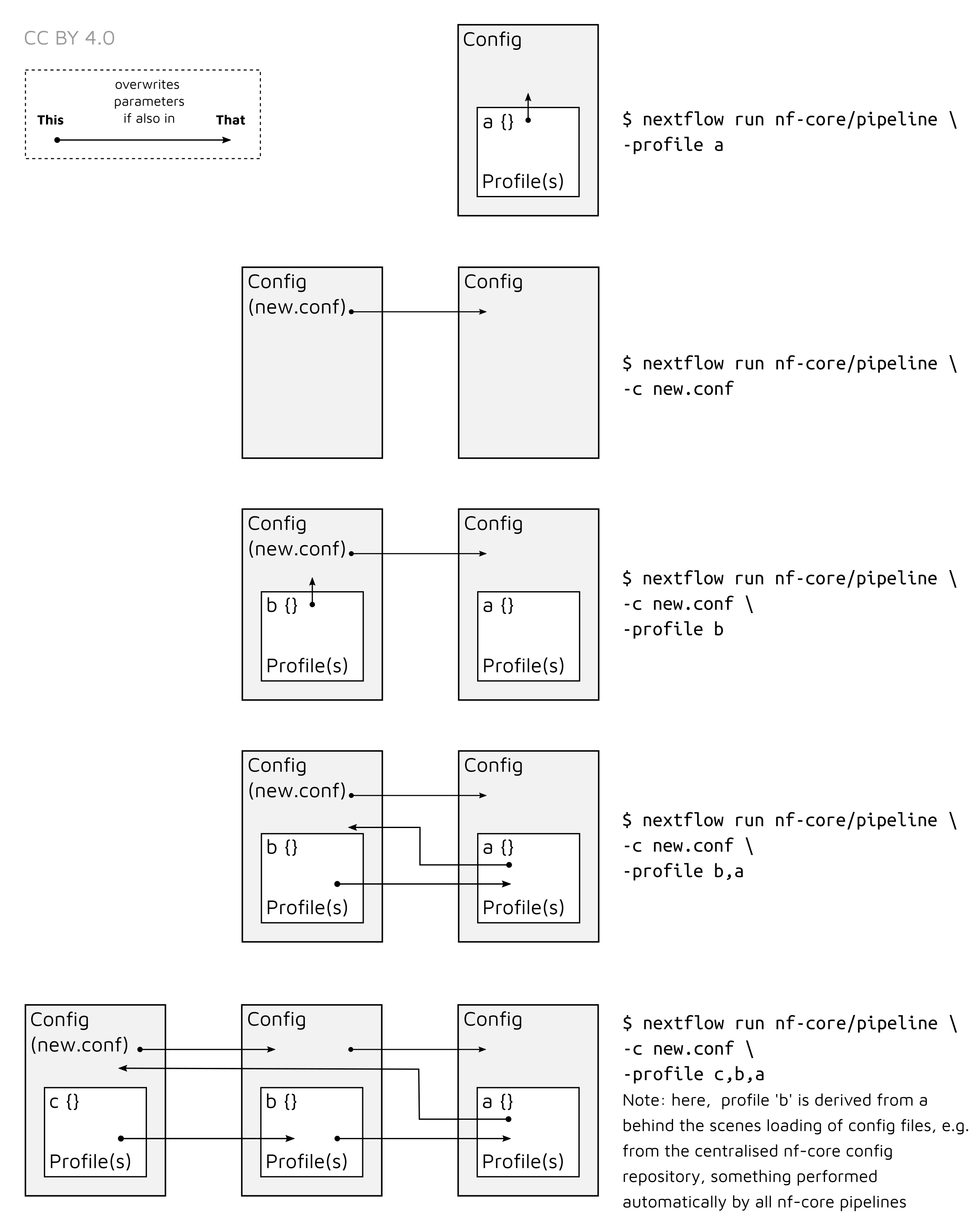
Using the example given in the background, if
the hpc_blue profile has the following pipeline parameters set
<...>mapper = 'bwamem'dedupper = 'markduplicates'<...>However, the profile old_dna has only the following parameter
<...>mapper = 'bwaaln'<...>Then running the pipeline with the profiles in the order of the following run command:
nextflow run nf-core/eager -c old_dna_profile.config -profile old_dna,hpc_blue <...>In the background, any parameters in the pipeline’s nextflow.config
(containing default parameters) will be overwritten by the
old_dna_profile.config. In addition, the old_dna profile will overwrite
any parameters set in the config but outside the profile definition of
old_dna_profile.config.
Therefore, the final profile used by your given run would look like:
<...>mapper = 'bwaaln'dedupper = 'markduplicates'<...>You can see here that markduplicates has not changed as originally defined in
the hpc_blue profile, but the mapper parameter has been changed from
bwamem to bwaaln, as specified in the old_dna profile.
The order of loading of different configuration files can be seen here:
| Loading Order | Configuration File |
|---|---|
| 1 | nextflow.config in your current directory, |
| 2 | (if using a script for nextflow run) a nextflow.config in the directory the script is located |
| 3 | config stored in your human directory under ~/.nextflow/ |
| 4 | <your_file>.config if you specify in the nextflow run command with -c |
| 5 | general nf-core institutional configurations stored at nf-core/configs |
| 6 | pipeline-specific nf-core institutional configurations at nf-core/configs |
This loading order of these .config files will not normally affect the
settings you use for the pipeline run itself; -profiles are normally more
important. However this is good to keep in mind when you need to debug profiles
if your run does not use the parameters you expect.
⚠️ It is also possible to ignore every configuration file other when specifying a custom
.configfile by using-C(capital C) instead of-c(which inherits previously specify parameters)
Another thing that is important to note is that if a specific profile is
specified in nextflow run, this replaces any ‘global’ parameter that is
specified within the config file (but outside a profile) itself - regardless
of profile order (see above).
For example, see the example adapted from the SHH nf-core/eager pipeline-specific configuration.
This pipeline-specific profile is automatically loaded if nf-core/eager detects
we are running eager, and that we specified the profile as shh.
// global 'fallback' parametersparams {  // Specific nf-core/configs params  config_profile_contact = 'James Fellows Yates (@jfy133)'  config_profile_description = 'nf-core/eager SHH profile provided by nf-core/configs'
  // default BWA   bwaalnn = 0.04   bwaalnl = 32}
}
// profile specific parametersprofiles {  pathogen_loose {    params {      config_profile_description = 'Pathogen (loose) MPI-SHH profile, provided by nf-core/configs.'      bwaalnn = 0.01      bwaalnl = 16    }  }}
If you run with nextflow run -profile shh to specify to use an
institutional-level nf-core config, the parameters will be read as --bwaalnn 0.04 and --bwaalnl 32 as these are the defaults ‘fall back’ params as
indicated in the example above.
If you specify as nextflow run -profile pathogen_loose,shh, as expected
Nextflow will resolve the two parameters as 0.01 and 16.
Importantly however, if you specify -profile shh,pathogen_loose the
pathogen_loose profile will still take precedence over just the
‘global’ params.
Equally, a process-level defined parameter (within the nf-core/eager code
itself) will take precedence over the fallback parameters in the config file.
This is also described in the Nextflow documentation
here
This is because selecting a profile will always take precedence over the
values specified in a config file, but outside of a profile.
Tutorial Profiles - Writing your own profile
We will now provide an example of how to write, use and share a project specific profile. We will use the example of Andrades Valtueña et al. 2016.
In it they used the original EAGER (v1) to map DNA from ancient DNA to the genome of the bacterium Yersinia pestis.
Now, we will generate a profile, that, if they were using nf-core/eager they could share with other researchers.
In the methods they described the following:
… reads mapped to Y. pestis CO92 reference with BWA aln (-l 16, -n 0.01, hereby referred to as non-UDG parameters). Reads with mapping quality scores lower than 37 were filtered out. PCR duplicates were removed with MarkDuplicates.“
Furthermore, in their ‘Table 1’ they say they used the NCBI Y. pestis genome ‘NC_003143.1’, which can be found on the NCBI FTP server at: https://ftp.ncbi.nlm.nih.gov/genomes/all/GCF/000/009/065/GCF_000009065.1_ASM906v1/GCF_000009065.1_ASM906v1_genomic.fna.gz
To make a profile with these parameters for use with nf-core/eager we first need to open a text editor, and define a Nextflow ‘profile’ block.
profiles {
}
Next we need to define the name of the profile. This is what we would write in
-profile. Lets call this AndradesValtuena2018.
profiles {  AndradesValtuena2018 {
  }}
Now we need to make a params ‘scope’. This means these are the parameters you
specifically pass to nf-core/eager itself (rather than Nextflow configuration
parameters).
You should generally not add non-params
scopes
in profiles for a specific project. This is because these will normally modify
the way the pipeline will run on the computer (rather than just nf-core/eager
itself, e.g. the scheduler/executor or maximum memory available), and thus not
allow other researchers to reproduce your analysis on their own
computer/clusters.
profiles {  AndradesValtuena2018 {    params {
    }  }}
Now, as a cool little trick, we can use a couple of nf-core specific parameters
that can help you keep track which profile you are using when running the
pipeline. The config_profile_description and config_profile_contact profiles
are displayed in the console log when running the pipeline. So you can use these
to check if your profile loaded as expected. These are free text boxes so you
can put what you like.
profiles { AndradesValtuena2018 { params { config_profile_description = 'non-UDG parameters used in Andrades Valtuena et al. 2018 Curr. Bio.' config_profile_contact = 'Aida Andrades Valtueña (@aidaanva)' } }}Now we can add the specific nf-core/eager parameters that will modify the mapping and deduplication parameters in nf-core/eager.
profiles { AndradesValtuena2018 { params { config_profile_description = 'non-UDG parameters used in Andrades Valtuena et al. 2018 Curr. Bio.' config_profile_contact = 'Aida Andrades Valtueña (@aidaanva)' fasta = 'https://ftp.ncbi.nlm.nih.gov/genomes/all/GCF/000/009/065/GCF_000009065.1_ASM906v1/GCF_000009065.1_ASM906v1_genomic.fna.gz' bwaalnn = 0.01 bwaalnl = 16 run_bam_filtering = true bam_mapping_quality_threshold = 37 dedupper = 'markduplicates' } }}Once filled in, we can save the file as AndradesValtuena2018.config. This you
can use yourself, or upload alongside your publication for others to use.
To use the profile you just need to specify the file containing the profile you wish to use, and then the profile itself.
For example, Aida (Andrades Valtueña) on her cluster sdag at the MPI-SHH
(shh) in Jena could run the following:
nextflow run nf-core/eager -c /<path>/<to>/AndradesValtuena2018.config -profile AndradesValtuena2018,sdag,shh --input '/<path>/<to>/<some_input>/' <...>Then a colleague at a different institution, such as the SciLifeLab, could run the same profile on the UPPMAX cluster in Uppsala with:
nextflow run nf-core/eager -c /<path>/<to>/AndradesValtuena2018.config -profile AndradesValtuena2018,uppmax --input '/<path>/<to>/<some_input>/' <...>And that’s all there is to it. Of course you should always check that there are no other ‘default’ parameters for your given pipeline are defined in any pipeline-specific or institutional profiles. This ensures that someone re-running the pipeline with your settings is as close to the nf-core/eager defaults as possible, and only settings specific to your given project are used. If there are ‘upstream’ defaults, you should explicitly specify these in your project profile.
Tutorial - How to set up nf-core/eager for human population genetics
Tutorial Human Pop-Gen - Introduction
This tutorial will give a basic example on how to set up nf-core/eager to perform initial screening of samples in the context of ancient human population genetics research.
⚠️ this tutorial does not describe how to install and set up nf-core/eager For this please see other documentation on the nf-co.re website.
We will describe how to set up mapping of ancient sequences against the human reference genome to allow sequencing and library quality-control, estimation of nuclear contamination, genetic sex determination, and production of random draw genotypes in eigenstrat format for a specific set of sites, to be used in further analysis. For this example, I will be using the 1240k SNP set. This SNP set was first described in Mathieson et al. 2015 and contains various positions along the genome that have been extensively genotyped in present-day and ancient populations, and are therefore useful for ancient population genetic analysis. Capture techniques are often used to enrich DNA libraries for fragments, that overlap these SNPs, as is being assumed has been performed in this example.
⚠️ Please be aware that the settings used in this tutorial may not use settings nor produce files you would actually use in ‘real’ analysis. The settings are only specified for demonstration purposes. Please consult the your colleagues, communities and the literature for optimal parameters.
Tutorial Human Pop-Gen - Preparation
Prior setting up the nf-core/eager run, we will need:
- Raw sequencing data in FASTQ format
- Reference genome in FASTA format, with associated pre-made
bwa,samtoolsandpicard SequenceDictionaryindices (however note these can be made for you with nf-core/eager, but this can make a pipeline run take much longer!) - A BED file with the positions of the sites of interest.
- An eigenstrat formatted
.snpfile for the positions of interest.
We should also ensure we have the very latest version of the nf-core/eager pipeline so we have all latest bugfixes etc. In this case we will be using nf-core/eager version 2.2.0. You should always check on the nf-core website whether a newer release has been made (particularly point releases e.g. 2.2.1).
nextflow pull nf-core/eager -r 2.2.0It is important to note that if you are planning on running multiple runs of nf-core/eager for a given project, that the version should be kept the same for all runs to ensure consistency in settings for all of your libraries.
Tutorial Human Pop-Gen - Inputs and Outputs
To start, lets make a directory where all your nf-core/eager related files for this run will go, and change into it.
mkdir projectX_preprocessing20200727cd projectX_preprocessing20200727The first part of constructing any nf-core/eager run is specifying a few generic parameters that will often be common across all runs. This will be which pipeline, version and profile we will use. We will also specify a unique name of the run to help us keep track of all the nf-core/eager runs you may be running.
nextflow run nf-core/eager \-r 2.2.0 \-profile sdag,shh,singularity \-name 'projectX_preprocessing20200727' \<...>For the -profile parameter, I have indicated that I wish to use Singularity as
my software container environment, and I will use the MPI-SHH institutional
config as listed on
nf-core/configs,
using the profile for the ‘sdag’ cluster. These profiles specify settings
optimised for the specific cluster/institution, such as maximum memory available
or which scheduler queues to submit to. More explanations about configs and
profiles can be seen in the nf-core
website and the profile
tutorial.
Next we need to specify our input data. nf-core/eager can accept input FASTQs files in two main ways, either with direct paths to files (with wildcards), or with a Tab-Separate-Value (TSV) file which contains the paths and extra metadata. In this example, we will use the TSV method, as to simulate a realistic use-case, such as receiving paired-end data from an Illumina NextSeq of double-stranded libraries. Illumina NextSeqs sequence a given library across four different ‘lanes’, so for each library you will receive four FASTQ files. The TSV input method is more useful for this context, as it allows ‘merging’ of these lanes after preprocessing prior mapping (whereas direct paths will consider each pair of FASTQ files as independent libraries/samples).
Our TSV file will look something like the following:
Sample_Name Library_ID Lane Colour_Chemistry SeqType Organism Strandedness UDG_Treatment R1 R2 BAMEGR001 EGR001.B0101.SG1 1 2 PE homo_sapiens double half ../../02-raw_data/EGR001.B0101.SG1.1/EGR001.B0101.SG1.1_S0_L001_R1_001.fastq.gz ../../02-raw_data/EGR001.B0101.SG1.1/EGR001.B0101.SG1.1_S0_L001_R2_001.fastq.gz NAEGR001 EGR001.B0101.SG1 2 2 PE homo_sapiens double half ../../02-raw_data/EGR001.B0101.SG1.1/EGR001.B0101.SG1.1_S0_L002_R1_001.fastq.gz ../../02-raw_data/EGR001.B0101.SG1.1/EGR001.B0101.SG1.1_S0_L002_R2_001.fastq.gz NAEGR001 EGR001.B0101.SG1 3 2 PE homo_sapiens double half ../../02-raw_data/EGR001.B0101.SG1.1/EGR001.B0101.SG1.1_S0_L003_R1_001.fastq.gz ../../02-raw_data/EGR001.B0101.SG1.1/EGR001.B0101.SG1.1_S0_L003_R2_001.fastq.gz NAEGR001 EGR001.B0101.SG1 4 2 PE homo_sapiens double half ../../02-raw_data/EGR001.B0101.SG1.1/EGR001.B0101.SG1.1_S0_L004_R1_001.fastq.gz ../../02-raw_data/EGR001.B0101.SG1.1/EGR001.B0101.SG1.1_S0_L004_R2_001.fastq.gz NAEGR001 EGR001.B0101.SG1 5 2 PE homo_sapiens double half ../../02-raw_data/EGR001.B0101.SG1.2/EGR001.B0101.SG1.2_S0_L001_R1_001.fastq.gz ../../02-raw_data/EGR001.B0101.SG1.2/EGR001.B0101.SG1.2_S0_L001_R2_001.fastq.gz NAEGR001 EGR001.B0101.SG1 6 2 PE homo_sapiens double half ../../02-raw_data/EGR001.B0101.SG1.2/EGR001.B0101.SG1.2_S0_L002_R1_001.fastq.gz ../../02-raw_data/EGR001.B0101.SG1.2/EGR001.B0101.SG1.2_S0_L002_R2_001.fastq.gz NAEGR001 EGR001.B0101.SG1 7 2 PE homo_sapiens double half ../../02-raw_data/EGR001.B0101.SG1.2/EGR001.B0101.SG1.2_S0_L003_R1_001.fastq.gz ../../02-raw_data/EGR001.B0101.SG1.2/EGR001.B0101.SG1.2_S0_L003_R2_001.fastq.gz NAEGR002 EGR002.B0201.SG1 8 2 PE homo_sapiens double half ../../02-raw_data/EGR001.B0101.SG1.2/EGR001.B0101.SG1.2_S0_L004_R1_001.fastq.gz ../../02-raw_data/EGR001.B0101.SG1.2/EGR001.B0101.SG1.2_S0_L004_R2_001.fastq.gz NAEGR002 EGR002.B0201.SG1 1 2 PE homo_sapiens double half ../../02-raw_data/EGR002.B0201.SG1.1/EGR002.B0201.SG1.1_S0_L001_R1_001.fastq.gz ../../02-raw_data/EGR002.B0201.SG1.1/EGR002.B0201.SG1.1_S0_L001_R2_001.fastq.gz NAEGR002 EGR002.B0201.SG1 2 2 PE homo_sapiens double half ../../02-raw_data/EGR002.B0201.SG1.1/EGR002.B0201.SG1.1_S0_L002_R1_001.fastq.gz ../../02-raw_data/EGR002.B0201.SG1.1/EGR002.B0201.SG1.1_S0_L002_R2_001.fastq.gz NAEGR002 EGR002.B0201.SG1 3 2 PE homo_sapiens double half ../../02-raw_data/EGR002.B0201.SG1.1/EGR002.B0201.SG1.1_S0_L003_R1_001.fastq.gz ../../02-raw_data/EGR002.B0201.SG1.1/EGR002.B0201.SG1.1_S0_L003_R2_001.fastq.gz NAEGR002 EGR002.B0201.SG1 4 2 PE homo_sapiens double half ../../02-raw_data/EGR002.B0201.SG1.1/EGR002.B0201.SG1.1_S0_L004_R1_001.fastq.gz ../../02-raw_data/EGR002.B0201.SG1.1/EGR002.B0201.SG1.1_S0_L004_R2_001.fastq.gz NAEGR002 EGR002.B0201.SG1 5 2 PE homo_sapiens double half ../../02-raw_data/EGR002.B0201.SG1.2/EGR002.B0201.SG1.2_S0_L001_R1_001.fastq.gz ../../02-raw_data/EGR002.B0201.SG1.2/EGR002.B0201.SG1.2_S0_L001_R2_001.fastq.gz NAEGR002 EGR002.B0201.SG1 6 2 PE homo_sapiens double half ../../02-raw_data/EGR002.B0201.SG1.2/EGR002.B0201.SG1.2_S0_L002_R1_001.fastq.gz ../../02-raw_data/EGR002.B0201.SG1.2/EGR002.B0201.SG1.2_S0_L002_R2_001.fastq.gz NAEGR002 EGR002.B0201.SG1 7 2 PE homo_sapiens double half ../../02-raw_data/EGR002.B0201.SG1.2/EGR002.B0201.SG1.2_S0_L003_R1_001.fastq.gz ../../02-raw_data/EGR002.B0201.SG1.2/EGR002.B0201.SG1.2_S0_L003_R2_001.fastq.gz NAEGR002 EGR002.B0201.SG1 8 2 PE homo_sapiens double half ../../02-raw_data/EGR002.B0201.SG1.2/EGR002.B0201.SG1.2_S0_L004_R1_001.fastq.gz ../../02-raw_data/EGR002.B0201.SG1.2/EGR002.B0201.SG1.2_S0_L004_R2_001.fastq.gz NAYou can see that we have a single line for each pair of FASTQ files representing
each Lane, but the Sample_Name and Library_ID columns identify and group
them together accordingly. Secondly, as we have NextSeq data, we have specified
we have 2 for Colour_Chemistry, which is important for downstream processing
(see below). See the nf-core/eager
parameter documentation above for more specifications on how to set up a
TSV file (e.g. why despite NextSeqs
only having 4 lanes, we go up to 8 in the example above).
Alongside our input TSV file, we will also specify the paths to our reference FASTA file and the corresponding indices.
nextflow run nf-core/eager \-r 2.2.0 \-profile sdag,shh,singularity \-name 'projectX_preprocessing20200727' \--input 'preprocessing20200727.tsv' \--fasta '../Reference/genome/hs37d5.fa' \--bwa_index '../Reference/genome/hs37d5/' \--fasta_index '../Reference/genome/hs37d5.fa.fai' \--seq_dict '../Reference/genome/hs37d5.dict' \<...>We specify the paths to each reference genome and it’s corresponding tool
specific index. Paths should always be encapsulated in quotes to ensure Nextflow
evaluates them, rather than your shell! Also note that as bwa generates
multiple index files, nf-core/eager takes a directory that must contain these
indices instead.
Note the difference between single and double
-parameters. The former represent Nextflow flags, while the latter are nf-core/eager specific flags.
Finally, we can also specify the output directory and the Nextflow work/
directory (which contains ‘intermediate’ working files and directories).
nextflow run nf-core/eager \-r 2.2.0 \-profile sdag,shh,singularity \-name 'projectX_preprocessing20200727' \--input 'preprocessing20200727.tsv' \`--fasta '../Reference/genome/hs37d5.fa' \--bwa_index '../Reference/genome/hs37d5/' \--fasta_index '../Reference/genome/hs37d5.fa.fai' \--seq_dict '../Reference/genome/hs37d5.dict' \--outdir './results/' \- w './work/' \<...>Tutorial Human Pop-Gen - Pipeline Configuration
Now that we have specified the input data, we can start moving onto specifying
settings for each different module we will be running. As mentioned above, we
are pretending to run with NextSeq data, which is generated with a two-colour
imaging technique. What this means is when you have shorter molecules than the
number of cycles of the sequencing chemistry, the sequencer will repeatedly see
‘G’ calls (no colour) at the last few cycles, and you get long poly-G ‘tails’ on
your reads. We therefore will turn on the poly-G clipping functionality offered
by fastp, and any pairs of files
indicated in the TSV file as having 2 in the Colour_Chemistry column will be
passed to fastp. We will not change the default minimum length of a poly-G
string to be clipped.
nextflow run nf-core/eager \-r 2.2.0 \-profile sdag,shh,singularity \-name 'projectX_preprocessing20200727' \--input 'preprocessing20200727.tsv' \--fasta '../Reference/genome/hs37d5.fa' \--bwa_index '../Reference/genome/hs37d5/' \--fasta_index '../Reference/genome/hs37d5.fa.fai' \--seq_dict '../Reference/genome/hs37d5.dict' \--outdir './results/' \- w './work/' \--complexity_filter_poly_g \<...>Since our input data is paired-end, we will be using DeDup for duplicate
removal, which takes into account both the start and end of a merged read before
flagging it as a duplicate. To ensure this happens works properly we first need
to disable base quality trimming of collapsed reads within Adapter Removal. To
do this, we will provide the option --preserve5p. Additionally, Dedup should
only be provided with merged reads, so we will need to provide the option
--mergedonly here as well. We can then specify which dedupper we want to use
with --dedupper.
nextflow run nf-core/eager \-r 2.2.0 \-profile sdag,shh,singularity \-name 'projectX_preprocessing20200727' \--input 'preprocessing20200727.tsv' \--fasta '../Reference/genome/hs37d5.fa' \--bwa_index '../Reference/genome/hs37d5/' \--fasta_index '../Reference/genome/hs37d5.fa.fai' \--seq_dict '../Reference/genome/hs37d5.dict' \--outdir './results/' \- w './work/' \--complexity_filter_poly_g \--preserve5p \--mergedonly \--dedupper 'dedup' \<...>We then need to specify the mapping parameters for this run. The default mapping
parameters of nf-core/eager are fine for the purposes of our run. Personally, I
like to set --bwaalnn to 0.01, (down from the default 0.04) which reduces
the stringency in the number of allowed mismatches between the aligned sequences
and the reference.
nextflow run nf-core/eager \-r 2.2.0 \-profile sdag,shh,singularity \-name 'projectX_preprocessing20200727' \--input 'preprocessing20200727.tsv' \--fasta '../Reference/genome/hs37d5.fa' \--bwa_index '../Reference/genome/hs37d5/' \--fasta_index '../Reference/genome/hs37d5.fa.fai' \--seq_dict '../Reference/genome/hs37d5.dict' \--outdir './results/' \- w './work/' \--complexity_filter_poly_g \--preserve5p \--mergedonly \--dedupper 'dedup' \--bwaalnn 0.01 \<...>We may also want to remove ambiguous sequences from our alignments, and also
remove off-target reads to speed up downstream processing (and reduce your
hard-disk footprint). We can do this with the samtools filter module to set a
mapping-quality filter (e.g. with a value of 25 to retain only slightly
ambiguous alignments that might occur from damage), and to indicate to discard
unmapped reads.
nextflow run nf-core/eager \-r 2.2.0 \-profile sdag,shh,singularity \-name 'projectX_preprocessing20200727' \--input 'preprocessing20200727.tsv' \--fasta '../Reference/genome/hs37d5.fa' \--bwa_index '../Reference/genome/hs37d5/' \--fasta_index '../Reference/genome/hs37d5.fa.fai' \--seq_dict '../Reference/genome/hs37d5.dict' \--outdir './results/' \- w './work/' \--complexity_filter_poly_g \--preserve5p \--mergedonly \--dedupper 'dedup' \--bwaalnn 0.01 \--run_bam_filtering \--bam_mapping_quality_threshold 25 \--bam_unmapped_type 'discard' \<...>Next, we will set up trimming of the mapped reads to alleviate the effects of DNA
damage during genotyping. To do this we will activate trimming with
--run_trim_bam. The libraries in this underwent ‘half’ UDG treatment. This
will generally restrict all remaining DNA damage to the first 2 base pairs of a
fragment. We will therefore use --bamutils_clip_half_udg_left and
--bamutils_clip_half_udg_right to trim 2bp on either side of each fragment.
nextflow run nf-core/eager \-r 2.2.0 \-profile sdag,shh,singularity \-name 'projectX_preprocessing20200727' \--input 'preprocessing20200727.tsv' \--fasta '../Reference/genome/hs37d5.fa' \--bwa_index '../Reference/genome/hs37d5/' \--fasta_index '../Reference/genome/hs37d5.fa.fai' \--seq_dict '../Reference/genome/hs37d5.dict' \--outdir './results/' \- w './work/' \--complexity_filter_poly_g \--preserve5p \--mergedonly \--dedupper 'dedup' \--bwaalnn 0.01 \--run_bam_filtering \--bam_mapping_quality_threshold 25 \--bam_unmapped_type 'discard' \--run_trim_bam \--bamutils_clip_half_udg_left 2 \--bamutils_clip_half_udg_right 2 \<...>To activate human sex determination (using
Sex.DetERRmine.py) we will
provide the option --run_sexdeterrmine. Additionally, we will provide
sexdeterrmine with the BED file of our SNPs of interest using the
--sexdeterrmine_bedfile flag. Here I will use the 1240k SNP set as an example.
This will cut down on computational time and also providing us with an
error bar around the relative coverage on the X and Y chromosomes.
nextflow run nf-core/eager \-r 2.2.0 \-profile sdag,shh,singularity \-name 'projectX_preprocessing20200727' \--input 'preprocessing20200727.tsv' \--fasta '../Reference/genome/hs37d5.fa' \--bwa_index '../Reference/genome/hs37d5/' \--fasta_index '../Reference/genome/hs37d5.fa.fai' \--seq_dict '../Reference/genome/hs37d5.dict' \--outdir './results/' \- w './work/' \--complexity_filter_poly_g \--preserve5p \--mergedonly \--dedupper 'dedup' \--bwaalnn 0.01 \--run_bam_filtering \--bam_mapping_quality_threshold 25 \--bam_unmapped_type 'discard' \--run_trim_bam \--bamutils_clip_half_udg_left 2 \--bamutils_clip_half_udg_right 2 \--run_sexdeterrmine \--sexdeterrmine_bedfile '../Reference/genome/1240k.sites.bed' \<...>Similarly, we will activate nuclear contamination estimation with
--run_nuclear_contamination. This process requires us to also specify the
contig name of the X chromosome in the reference genome we are using with
--contamination_chrom_name. Here, we are using hs37d5, where the X chromosome
is simply named ‘X’.
nextflow run nf-core/eager \-r 2.2.0 \-profile sdag,shh,singularity \-name 'projectX_preprocessing20200727' \--input 'preprocessing20200727.tsv' \--fasta '../Reference/genome/hs37d5.fa' \--bwa_index '../Reference/genome/hs37d5/' \--fasta_index '../Reference/genome/hs37d5.fa.fai' \--seq_dict '../Reference/genome/hs37d5.dict' \--outdir './results/' \- w './work/' \--complexity_filter_poly_g \--preserve5p \--mergedonly \--dedupper 'dedup' \--bwaalnn 0.01 \--run_bam_filtering \--bam_mapping_quality_threshold 25 \--bam_unmapped_type 'discard' \--run_trim_bam \--bamutils_clip_half_udg_left 2 \--bamutils_clip_half_udg_right 2 \--run_sexdeterrmine \--sexdeterrmine_bedfile '../Reference/genome/1240k.sites.bed' \--run_nuclear_contamination \--contamination_chrom_name 'X' \<...>Because nuclear contamination estimates can only be provided for males, it is
possible that we will need to get mitochondrial DNA contamination estimates for
any females in our dataset. This cannot be done within nf-core/eager (v2.2.0)
and we will need to do this manually at a later time. However, mtDNA
contamination estimates have been shown to only be reliable for nuclear
contamination when the ratio of mitochondrial to nuclear reads is low
(Furtwängler et al. 2018). We can
have nf-core/eager calculate that ratio for us with --run_mtnucratio, and
providing the name of the mitochondrial DNA contig in our reference genome with
--mtnucratio_header. Within hs37d5, the mitochondrial contig is named ‘MT’.
nextflow run nf-core/eager \-r 2.2.0 \-profile sdag,shh,singularity \-name 'projectX_preprocessing20200727' \--input 'preprocessing20200727.tsv' \--fasta '../Reference/genome/hs37d5.fa' \--bwa_index '../Reference/genome/hs37d5/' \--fasta_index '../Reference/genome/hs37d5.fa.fai' \--seq_dict '../Reference/genome/hs37d5.dict' \--outdir './results/' \- w './work/' \--complexity_filter_poly_g \--preserve5p \--mergedonly \--dedupper 'dedup' \--bwaalnn 0.01 \--run_bam_filtering \--bam_mapping_quality_threshold 25 \--bam_unmapped_type 'discard' \--run_trim_bam \--bamutils_clip_half_udg_left 2 \--bamutils_clip_half_udg_right 2 \--run_sexdeterrmine \--sexdeterrmine_bedfile '../Reference/genome/1240k.sites.bed' \--run_nuclear_contamination \--contamination_chrom_name 'X' \--run_mtnucratio \--mtnucratio_header 'MT' \<...>Finally, we need to specify genotyping parameters. First, we need to activate
genotyping with --run_genotyping. It is also important to specify we wish to
use the trimmed data for genotyping, to avoid the effects of DNA damage. To
do this, we will specify the --genotyping_source as 'trimmed'. Then we can
specify the genotyping tool to use with --genotyping_tool. We will be using
'pileupCaller' to produce random draw genotypes in eigenstrat format. For this
process we will need to specify a BED file of the sites of interest (the same as
before) with --pileupcaller_bedfile, as well as an eigenstrat formatted .snp
file of these sites that is specified with --pileupcaller_snpfile.
nextflow run nf-core/eager \-r 2.2.0 \-profile sdag,shh,singularity \-name 'projectX_preprocessing20200727' \--input 'preprocessing20200727.tsv' \--fasta '../Reference/genome/hs37d5.fa' \--bwa_index '../Reference/genome/hs37d5/' \--fasta_index '../Reference/genome/hs37d5.fa.fai' \--seq_dict '../Reference/genome/hs37d5.dict' \--outdir './results/' \- w './work/' \--complexity_filter_poly_g \--preserve5p \--mergedonly \--dedupper 'dedup' \--bwaalnn 0.01 \--run_bam_filtering \--bam_mapping_quality_threshold 25 \--bam_unmapped_type 'discard' \--run_trim_bam \--bamutils_clip_half_udg_left 2 \--bamutils_clip_half_udg_right 2 \--run_sexdeterrmine \--sexdeterrmine_bedfile '../Reference/genome/1240k.sites.bed' \--run_nuclear_contamination \--contamination_chrom_name 'X' \--run_mtnucratio \--mtnucratio_header 'MT' \--run_genotyping \--genotyping_source 'trimmed' \--genotyping_tool 'pileupcaller' \--pileupcaller_bedfile '../Reference/genome/1240k.sites.bed' \--pileupcaller_snpfile '../Datasets/1240k/1240k.snp'With this, we are ready to submit! If running on a remote cluster/server, Make
sure to run this in a screen session or similar, so that if you get a ssh
signal drop or want to log off, Nextflow will not crash.
Tutorial Human Pop-Gen - Results
Assuming the run completed without any crashes (if problems do occur, check
against #usage that all parameters are as expected, or
check the FAQ), we can now check our results in
results/.
Tutorial Human Pop-Gen - MultiQC Report
In here there are many different directories containing different output files.
The first directory to check is the MultiQC/ directory. You should
find a multiqc_report.html file. You will need to view this in a web browser,
so I recommend either mounting your server to your file browser, or downloading
it to your own local machine (PC/Laptop etc.).
Once you’ve opened this you can go through each section and evaluate all the results. You will likely want to check these for artefacts (e.g. weird damage patterns on the human DNA, or weirdly skewed coverage distributions).
For example, I normally look for things like:
General Stats Table:
- Do I see the expected number of raw sequencing reads (summed across each set of FASTQ files per library) that was requested for sequencing?
- Does the percentage of trimmed reads look normal for aDNA, and do lengths after trimming look short as expected of aDNA?
- Does ClusterFactor or ‘Dups’ look high (e.g. >2 or >10% respectively) suggesting over-amplified or badly preserved samples?
- Do the mapped reads show increased frequency of C>Ts on the 5’ end of molecules?
- Is the number of SNPs used for nuclear contamination really low for any individuals (e.g. < 100)? If so, then the estimates might not be very accurate.
FastQC (pre-AdapterRemoval):
- Do I see any very early drop off of sequence quality scores suggesting a problematic sequencing run?
- Do I see outlier GC content distributions?
- Do I see high sequence duplication levels?
AdapterRemoval:
- Do I see high numbers of singletons or discarded read pairs?
FastQC (post-AdapterRemoval):
- Do I see improved sequence quality scores along the length of reads?
- Do I see reduced adapter content levels?
Samtools Flagstat (pre/post Filter):
- Do I see outliers, e.g. with unusually high levels of human DNA, (indicative of contamination) that require downstream closer assessment? Are your samples exceptionally preserved? If not, a value higher than e.g. 50% might require your attention.
DeDup/Picard MarkDuplicates:
- Do I see large numbers of duplicates being removed, possibly indicating over-amplified or badly preserved samples?
DamageProfiler:
- Do I see evidence of damage on human DNA?
- High numbers of mapped reads but no damage may indicate significant modern contamination.
- Was the read trimming I specified enough to overcome damage effects?
SexDetERRmine:
- Do the relative coverages on the X and Y chromosome fall within the expected areas of the plot?
- Do all individuals have enough data for accurate sex determination?
- Do the proportions of autosomal/X/Y reads make sense? If there is an overrepresentation of reads within one bin, is the data enriched for that bin?
Detailed documentation and descriptions for all MultiQC modules can be seen in the the ‘Documentation’ folder of the results directory or here in the output documentation
If you’re happy everything looks good in terms of sequencing, we then look at specific directories to find any files you might want to use for downstream processing.
Note that when you get back to writing up your publication, all the versions of the tools can be found under the ‘nf-core/eager Software Versions’ section of the MultiQC report. But be careful! All tools in the container are listed, so you may have to remove some of them that you didn’t actually use in the set up.
For example, in this example, we have used: Nextflow, nf-core/eager, FastQC, AdapterRemoval, fastP, BWA, Samtools, endorS.py, DeDup, Qualimap, PreSeq, DamageProfiler, bamUtil, sexdeterrmine, angsd, MTNucRatioCalculator, sequenceTools, and MultiQC.
Citations to all used tools can be seen here
Tutorial Human Pop-Gen - Files for Downstream Analysis
You will find the eigenstrat dataset containing the random draw genotypes of
your run in the genotyping/ directory. Genotypes from double stranded
libraries, like the ones in this example, are found in the dataset
pileupcaller.double.{geno,snp,ind}.txt, while genotypes for any single
stranded libraries will instead be in pileupcaller.single.{geno,snp,ind}.txt.
Tutorial Human Pop-Gen - Clean up
Finally, I would recommend cleaning up your work/ directory of any
intermediate files (if your -profile does not already do so). You can do this
by going to above your results/ and work/ directory, e.g.
cd /<path>/<to>/projectX_preprocessing20200727and running
nextflow clean -f -kTutorial Human Pop-Gen - Summary
In this this tutorial we have described an example on how to set up an nf-core/eager run to preprocess human aDNA for population genetic studies, preform some simple quality control checks, and generate random draw genotypes for downstream analysis of the data. Additionally, we described what to look for in the run summary report generated by MultiQC and where to find output files that can be used for downstream analysis.
Tutorial - How to set up nf-core/eager for metagenomic screening
Tutorial Metagenomics - Introduction
The field of archaeogenetics is now expanding out from analysing the genomes of single organisms but to whole communities of taxa. One particular example is of human associated microbiomes, as preserved in ancient palaeofaeces (gut) or dental calculus (oral). This tutorial will give a basic example on how to set up nf-core/eager to perform initial screening of samples in the context of ancient microbiome research.
⚠️ this tutorial does not describe how to install and set up nf-core/eager For this please see other documentation on the nf-co.re website.
We will describe how to set up mapping of ancient dental calculus samples against the human reference genome to allow sequencing and library quality-control, but additionally perform taxonomic profiling of the off-target reads from this mapping using MALT, and perform aDNA authentication with HOPS.
⚠️ Please be aware that the settings used in this tutorial may not use settings nor produce files you would actually use in ‘real’ analysis. The settings are only specified for demonstration purposes. Please consult the your colleagues, communities and the literature for optimal parameters.
Tutorial Metagenomics - Preparation
Prior setting up an nf-core/eager run for metagenomic screening, we will need:
- Raw sequencing data in FASTQ format
- Reference genome in FASTA format, with associated pre-made
bwa,samtoolsandpicard SequenceDictionaryindices - A MALT database of your choice (see MALT manual for set-up)
- A list of (NCBI) taxa containing well-known taxa of your microbiome (see below)
- HOPS resources
.mapand.trefiles (available here)
We should also ensure we have the very latest version of the nf-core/eager pipeline so we have all latest bugfixes etc. In this case we will be using nf-core/eager version 2.2.0. You should always check on the nf-core website whether a newer release has been made (particularly point releases e.g. 2.2.1).
nextflow pull nf-core/eager -r 2.2.0It is important to note that if you are planning on running multiple runs of nf-core/eager for a given project, that the version should be kept the same for all runs to ensure consistency in settings for all of your libraries.
Tutorial Metagenomics - Inputs and Outputs
To start, lets make a directory where all your nf-core/eager related files for this run will go, and change into it.
mkdir projectX_screening20200720cd projectX_screening20200720The first part of constructing any nf-core/eager run is specifying a few generic parameters that will often be common across all runs. This will be which pipeline, version and profile we will use. We will also specify a unique name of the run to help us keep track of all the nf-core/eager runs you may be running.
nextflow run nf-core/eager \-r 2.2.0 \-profile sdag,shh,singularity \-name 'projectX_screening20200720' \<...>For the -profile parameter, I have indicated that I wish to use Singularity as
my software container environment, and I will use the MPI-SHH institutional
config as listed on
nf-core/configs,
and using the profile for the ‘sdag’ cluster. These profiles specify settings
optimised for the specific cluster/institution, such as maximum memory available
or which scheduler queues to submit to. More explanations about configs and
profiles can be seen in the nf-core
website and the profile
tutorial.
Next we need to specify our input data. nf-core/eager can accept input FASTQs files in two main ways, either with direct paths to files (with wildcards), or with a Tab-Separate-Value (TSV) file which contains the paths and extra metadata. In this example, we will use the TSV method, as to simulate a realistic use-case, such as receiving paired-end data from an Illumina NextSeq of double-stranded libraries. Illumina NextSeqs sequence a given library across four different ‘lanes’, so for each library you will receive four FASTQ files. The TSV input method is more useful for this context, as it allows ‘merging’ of these lanes after preprocessing prior mapping (whereas direct paths will consider each pair of FASTQ files as independent libraries/samples).
Our TSV file will look something like the following:
Sample_Name Library_ID Lane Colour_Chemistry SeqType Organism Strandedness UDG_Treatment R1 R2 BAMEGR001 EGR001.B0101.SG1 1 2 PE homo_sapiens double half ../../02-raw_data/EGR001.B0101.SG1.1/EGR001.B0101.SG1.1_S0_L001_R1_001.fastq.gz ../../02-raw_data/EGR001.B0101.SG1.1/EGR001.B0101.SG1.1_S0_L001_R2_001.fastq.gz NAEGR001 EGR001.B0101.SG1 2 2 PE homo_sapiens double half ../../02-raw_data/EGR001.B0101.SG1.1/EGR001.B0101.SG1.1_S0_L002_R1_001.fastq.gz ../../02-raw_data/EGR001.B0101.SG1.1/EGR001.B0101.SG1.1_S0_L002_R2_001.fastq.gz NAEGR001 EGR001.B0101.SG1 3 2 PE homo_sapiens double half ../../02-raw_data/EGR001.B0101.SG1.1/EGR001.B0101.SG1.1_S0_L003_R1_001.fastq.gz ../../02-raw_data/EGR001.B0101.SG1.1/EGR001.B0101.SG1.1_S0_L003_R2_001.fastq.gz NAEGR001 EGR001.B0101.SG1 4 2 PE homo_sapiens double half ../../02-raw_data/EGR001.B0101.SG1.1/EGR001.B0101.SG1.1_S0_L004_R1_001.fastq.gz ../../02-raw_data/EGR001.B0101.SG1.1/EGR001.B0101.SG1.1_S0_L004_R2_001.fastq.gz NAEGR001 EGR001.B0101.SG1 5 2 PE homo_sapiens double half ../../02-raw_data/EGR001.B0101.SG1.2/EGR001.B0101.SG1.2_S0_L001_R1_001.fastq.gz ../../02-raw_data/EGR001.B0101.SG1.2/EGR001.B0101.SG1.2_S0_L001_R2_001.fastq.gz NAEGR001 EGR001.B0101.SG1 6 2 PE homo_sapiens double half ../../02-raw_data/EGR001.B0101.SG1.2/EGR001.B0101.SG1.2_S0_L002_R1_001.fastq.gz ../../02-raw_data/EGR001.B0101.SG1.2/EGR001.B0101.SG1.2_S0_L002_R2_001.fastq.gz NAEGR001 EGR001.B0101.SG1 7 2 PE homo_sapiens double half ../../02-raw_data/EGR001.B0101.SG1.2/EGR001.B0101.SG1.2_S0_L003_R1_001.fastq.gz ../../02-raw_data/EGR001.B0101.SG1.2/EGR001.B0101.SG1.2_S0_L003_R2_001.fastq.gz NAEGR002 EGR002.B0201.SG1 8 2 PE homo_sapiens double half ../../02-raw_data/EGR001.B0101.SG1.2/EGR001.B0101.SG1.2_S0_L004_R1_001.fastq.gz ../../02-raw_data/EGR001.B0101.SG1.2/EGR001.B0101.SG1.2_S0_L004_R2_001.fastq.gz NAEGR002 EGR002.B0201.SG1 1 2 PE homo_sapiens double half ../../02-raw_data/EGR002.B0201.SG1.1/EGR002.B0201.SG1.1_S0_L001_R1_001.fastq.gz ../../02-raw_data/EGR002.B0201.SG1.1/EGR002.B0201.SG1.1_S0_L001_R2_001.fastq.gz NAEGR002 EGR002.B0201.SG1 2 2 PE homo_sapiens double half ../../02-raw_data/EGR002.B0201.SG1.1/EGR002.B0201.SG1.1_S0_L002_R1_001.fastq.gz ../../02-raw_data/EGR002.B0201.SG1.1/EGR002.B0201.SG1.1_S0_L002_R2_001.fastq.gz NAEGR002 EGR002.B0201.SG1 3 2 PE homo_sapiens double half ../../02-raw_data/EGR002.B0201.SG1.1/EGR002.B0201.SG1.1_S0_L003_R1_001.fastq.gz ../../02-raw_data/EGR002.B0201.SG1.1/EGR002.B0201.SG1.1_S0_L003_R2_001.fastq.gz NAEGR002 EGR002.B0201.SG1 4 2 PE homo_sapiens double half ../../02-raw_data/EGR002.B0201.SG1.1/EGR002.B0201.SG1.1_S0_L004_R1_001.fastq.gz ../../02-raw_data/EGR002.B0201.SG1.1/EGR002.B0201.SG1.1_S0_L004_R2_001.fastq.gz NAEGR002 EGR002.B0201.SG1 5 2 PE homo_sapiens double half ../../02-raw_data/EGR002.B0201.SG1.2/EGR002.B0201.SG1.2_S0_L001_R1_001.fastq.gz ../../02-raw_data/EGR002.B0201.SG1.2/EGR002.B0201.SG1.2_S0_L001_R2_001.fastq.gz NAEGR002 EGR002.B0201.SG1 6 2 PE homo_sapiens double half ../../02-raw_data/EGR002.B0201.SG1.2/EGR002.B0201.SG1.2_S0_L002_R1_001.fastq.gz ../../02-raw_data/EGR002.B0201.SG1.2/EGR002.B0201.SG1.2_S0_L002_R2_001.fastq.gz NAEGR002 EGR002.B0201.SG1 7 2 PE homo_sapiens double half ../../02-raw_data/EGR002.B0201.SG1.2/EGR002.B0201.SG1.2_S0_L003_R1_001.fastq.gz ../../02-raw_data/EGR002.B0201.SG1.2/EGR002.B0201.SG1.2_S0_L003_R2_001.fastq.gz NAEGR002 EGR002.B0201.SG1 8 2 PE homo_sapiens double half ../../02-raw_data/EGR002.B0201.SG1.2/EGR002.B0201.SG1.2_S0_L004_R1_001.fastq.gz ../../02-raw_data/EGR002.B0201.SG1.2/EGR002.B0201.SG1.2_S0_L004_R2_001.fastq.gz NAYou can see that we have a single line for each pair of FASTQ files representing
each Lane, but the Sample_Name and Library_ID columns identify and group
them together accordingly. Secondly, as we have NextSeq data, we have specified
we have 2 for Colour_Chemistry, which is important for downstream processing
(see below). The other columns are less important for this particular context of
metagenomic screening. See the nf-core/eager usage
documentation for more specifications on how to set up a TSV file (e.g. why
despite NextSeqs only having 4 lanes, we go up to 8 in the example above).
Alongside our input TSV file, we will also specify the paths to our reference FASTA file and the corresponding indices.
nextflow run nf-core/eager \-r 2.2.0 \-profile sdag,shh,singularity \-name 'projectX_screening20200720' \--input 'screening20200720.tsv' \--fasta '../Reference/genome/GRCh38.fa' \--bwa_index '../Reference/genome/GRCh38/' \--fasta_index '../Reference/genome/GRCh38.fa.fai' \--seq_dict '../Reference/genome/GRCh38.dict' \<...>We specify the paths to each reference genome and it’s corresponding tool
specific index. Paths should always be encapsulated in quotes to ensure Nextflow
evaluates them, rather than your shell! Also note that as bwa generates
multiple index files, nf-core/eager takes a directory that must contain these
indices instead.
Note the difference between single and double
-parameters. The former represent Nextflow flags, while double are nf-core/eager specific flags.
Finally, we can also specify the output directory and the Nextflow work/
directory (which contains ‘intermediate’ working files and directories).
nextflow run nf-core/eager \-r 2.2.0 \-profile sdag,shh,singularity \-name 'projectX_screening20200720' \--input 'screening20200720.tsv' \--fasta '../Reference/genome/GRCh38.fa' \--bwa_index '../Reference/genome/GRCh38/' \--fasta_index '../Reference/genome/GRCh38.fa.fai' \--seq_dict '../Reference/genome/GRCh38.dict' \--outdir './results/' \- w './work/' \<...>Tutorial Metagenomics - Pipeline Configuration
Now that we have specified the input data, we can start moving onto specifying
settings for each different module we will be running. As mentioned above, we
are pretending to run with NextSeq data, which is generated with a two-colour
imaging technique. What this means is when you have shorter molecules than the
number of cycles of the sequencing chemistry, the sequencer will repeatedly see
‘G’ calls (no colour) at the last few cycles, and you get long poly-G ‘tails’ on
your reads. We therefore will turn on the poly-G clipping functionality offered
by fastp, and any pairs of files
indicated in the TSV file as having 2 in the Colour_Chemistry column will be
passed to fastp. We will not change the default minimum length of a poly-G
string to be clipped.
nextflow run nf-core/eager \-r 2.2.0 \-profile sdag,shh,singularity \-name 'projectX_screening20200720' \--input 'screening20200720.tsv' \--fasta '../Reference/genome/GRCh38.fa' \--bwa_index '../Reference/genome/GRCh38/' \--fasta_index '../Reference/genome/GRCh38.fa.fai' \--seq_dict '../Reference/genome/GRCh38.dict' \--outdir './results/' \- w './work/' \--complexity_filter_poly_g \<...>We will keep the default settings for mapping etc. against the reference genome as we will only use this for sequencing quality control, however we now need to specify that we want to run metagenomic screening. To do this we firstly need to tell nf-core/eager what to do with the off target reads from the mapping.
nextflow run nf-core/eager \-r 2.2.0 \-profile sdag,shh,singularity \-name 'projectX_screening20200720' \--input 'screening20200720.tsv' \--fasta '../Reference/genome/GRCh38.fa' \--bwa_index '../Reference/genome/GRCh38/' \--fasta_index '../Reference/genome/GRCh38.fa.fai' \--seq_dict '../Reference/genome/GRCh38.dict' \--outdir './results/' \- w './work/' \--complexity_filter_poly_g \--run_bam_filtering \--bam_unmapped_type 'fastq' \<...>nf-core/eager will now take all unmapped reads after mapping and convert the BAM
file back to FASTQ, which can be accepted by MALT. But of course, we also then
need to tell nf-core/eager we actually want to run MALT. We will also specify
the location of the pre-built database and which ‘min support’
method we want to use (this specifies the minimum number of alignments is needed
to a particular taxonomic node to be ‘kept’ in the MALT output files). Otherwise
we will keep all other parameters as default. For example using BlastN mode,
requiring a minimum of 85% identity, requiring at least 0.01% alignments for a
taxon to be saved (as specified with the --malt_min_support_mode). More
documentation describing each parameters can be seen in the usage
documentation
nextflow run nf-core/eager \-r 2.2.0 \-profile sdag,shh,singularity \-name 'projectX_screening20200720' \--input 'screening20200720.tsv' \--fasta '../Reference/genome/GRCh38.fa' \--bwa_index '../Reference/genome/GRCh38/' \--fasta_index '../Reference/genome/GRCh38.fa.fai' \--seq_dict '../Reference/genome/GRCh38.dict' \--outdir './results/' \- w './work/' \--complexity_filter_poly_g \--run_bam_filtering \--bam_unmapped_type 'fastq' \--run_metagenomic_screening \--metagenomic_tool 'malt' \--database '../Reference/database/refseq-bac-arch-homo-2018_11' \--malt_min_support_mode 'percent' \<...>Finally, to help quickly assess whether we our sample has taxa that are known to exist in (modern samples of) our expected microbiome, and that these alignments have indicators of true aDNA, we will run ‘maltExtract’ of the HOPS pipeline.
nextflow run nf-core/eager \-r 2.2.0 \-profile sdag,shh,singularity \-name 'projectX_screening20200720' \--input 'screening20200720.tsv' \--fasta '../Reference/genome/GRCh38.fa' \--bwa_index '../Reference/genome/GRCh38/' \--fasta_index '../Reference/genome/GRCh38.fa.fai' \--seq_dict '../Reference/genome/GRCh38.dict' \--outdir './results/' \- w './work/' \--complexity_filter_poly_g \--run_bam_filtering \--bam_unmapped_type 'fastq' \--run_metagenomic_screening \--metagenomic_tool 'malt' \--database '../Reference/database/refseq-bac-arch-homo-2018_11' \--malt_min_support_mode 'percent' \--run_maltextract \--maltextract_taxon_list '../Reference/taxa_list/core_genera-anthropoids_hominids_panhomo-20180131.txt' \--maltextract_ncbifiles '../Reference/hops' \--maltextract_destackingoffIn the last parameters above we’ve specified the path to our list of taxa. This contains something like (for oral microbiomes):
ActinomycesStreptococcusTannerellaPorphyromonasWe have also specified the path to the HOPS resources downloaded earlier, and that I want to turn off ‘destacking’ (removal of any read that overlaps the positions of another - something only recommended to keep on when you have high coverage data).
With this, we are ready to submit! If running on a remote cluster/server, Make
sure to run this in a screen session or similar, so that if you get a ssh
signal drop or want to log off, Nextflow will not crash.
Tutorial Metagenomics - Results
Assuming the run completed without any crashes (if problems do occur, check
against usage that all parameters are as expected, or check
the FAQ), we can now check our results in
results/.
Tutorial Metagenomics - MultiQC Report
In here there are many different directories containing different output files.
The first directory to check is the MultiQC/ directory. You should
find a multiqc_report.html file. You will need to view this in a web browser,
so I recommend either mounting your server to your file browser, or downloading
it to your own local machine (PC/Laptop etc.).
Once you’ve opened this you can go through each section and evaluate all the results. You will likely not want to concern yourself too much with anything after MALT - however you should check these for other artefacts (e.g. weird damage patterns on the human DNA, or weirdly skewed coverage distributions).
For example, I normally look for things like:
General Stats Table:
- Do I see the expected number of raw sequencing reads (summed across each set of FASTQ files per library) that was requested for sequencing?
- Does the percentage of trimmed reads look normal for aDNA, and do lengths after trimming look short as expected of aDNA?
- Does ClusterFactor or ‘Dups’ look high suggesting over-amplified or badly preserved samples (e.g. >2 or >10% respectively - however given this is on the human reads this is just a rule of thumb and may not reflect the quality of the metagenomic profile) ?
- Does the human DNA show increased frequency of C>Ts on the 5’ end of molecules?
FastQC (pre-AdapterRemoval):
- Do I see any very early drop off of sequence quality scores suggesting problematic sequencing run?
- Do I see outlier GC content distributions?
- Do I see high sequence duplication levels?
AdapterRemoval:
- Do I see high numbers of singletons or discarded read pairs?
FastQC (post-AdapterRemoval):
- Do I see improved sequence quality scores along the length of reads?
- Do I see reduced adapter content levels?
MALT:
- Do I have a reasonable level of mappability?
- Somewhere between 10-30% can be pretty normal for aDNA, whereas e.g. <1% requires careful manual assessment
- Do I have a reasonable taxonomic assignment success?
- You hope to have a large number of the mapped reads (from the mappability plot) that also have taxonomic assignment.
Samtools Flagstat (pre/post Filter):
- Do I see outliers, e.g. with unusually high levels of human DNA, (indicative of contamination) that require downstream closer assessment?
DeDup/Picard MarkDuplicates:
- Do I see large numbers of duplicates being removed, possibly indicating over-amplified or badly preserved samples?
DamageProfiler:
- Do I see evidence of damage on human DNA? Note this is just a
rule-of-thumb/corroboration of any signals you might find in the metagenomic
screening and not essential.
- If you have high numbers of human DNA reads but no damage may indicate significant modern contamination.
Detailed documentation and descriptions for all MultiQC modules can be seen in the the ‘Documentation’ folder of the results directory or here in the output documentation
If you’re happy everything looks good in terms of sequencing, we then look at specific directories to find any files you might want to use for downstream processing.
Note that when you get back to writing up your publication, all the versions of the tools can be found under the ‘nf-core/eager Software Versions’ section of the MultiQC report. Note that all tools in the container are listed, so you may have to remove some of them that you didn’t actually use in the set up.
For example, in the example above, we have used: Nextflow, nf-core/eager, FastQC, AdapterRemoval, fastP, BWA, Samtools, endorS.py, Picard Markduplicates, Qualimap, PreSeq, DamageProfiler, MALT, MaltExtract and MultiQC.
Citations to all used tools can be seen here
Tutorial Metagenomics - Files for Downstream Analysis
If you wanted to look at the output of MALT more closely, such as in the GUI
based tool
MEGAN6,
you can find the .rma6 files that is accepted by MEGAN under
metagenomic_classification/malt/. The log file containing the information
printed to screen while MALT is running can also be found in this directory.
As we ran the HOPS pipeline (primarily the MaltExtract tool), we can look in
MaltExtract/results/ to find all the corresponding output files for the
authentication validation of the metagenomic screening (against the taxa you
specified in your --maltextract_taxon_list). First you can check the
heatmap_overview_Wevid.pdf summary PDF from HOPS (again you will need to
either mount the server or download), but to get the actual per-sample/taxon
damage patterns etc., you can look in pdf_candidate_profiles. In some cases
there maybe valid results that the HOPS ‘postprocessing’ script doesn’t pick up.
In these cases you can go into the default directory to find all the raw text
files which you can use to visualise and assess the authentication results
yourself.
Finally, if you want to re-run the taxonomic classification with a new database
or tool, to find the raw fastq/ files containing only unmapped reads that went
into MALT, you should go into samtools/filter. In here you will find files
ending in unmapped.fastq.gz for each library.
Tutorial Metagenomics - Clean up
Finally, I would recommend cleaning up your work/ directory of any
intermediate files (if your -profile does not already do so). You can do this
by going to above your results/ and work/ directory, e.g.
cd /<path>/<to>/projectX_screening20200720and running
nextflow clean -f -kTutorial Metagenomics - Summary
In this this tutorial we have described an example on how to set up a metagenomic screening run of ancient microbiome samples. We have covered how to set up nf-core/eager to extract off-target reads in a form that can be used for MALT, and how to additionally run HOPS to authenticate expected taxa to be found in the human oral microbiome. Finally we have also described what to look for in the MultiQC run summary report and where to find output files that can be used for downstream analysis.
Tutorial - How to set up nf-core/eager for pathogen genomics
Tutorial Pathogen Genomics - Introduction
This tutorial will give a basic example on how to set up nf-core/eager to perform bacterial genome reconstruction from samples in the context of ancient pathogenomic research.
⚠️ this tutorial does not describe how to install and set-up nf-core/eager For this please see other documentation on the nf-co.re website.
We will describe how to set up mapping ancient pathogen samples against the reference of a targeted organism genome, to check sequencing and library quality-control, calculation of depth and breath of coverage, check for damage profiles, feature-annotation statistics (e.g. for gene presence and absence), SNP calling, and producing an SNP alignment for its usage in downstream phylogenetic analysis.
I will use as an example data from Andrades Valtueña et al 2017, who retrieved Late Neolithic/Bronze Age Yersinia pestis genomes. This data is very large shotgun data and is not ideal for testing, so running on your own data is recommended as otherwise running this data will require a lot of computing resources and time. However, note the same procedure can equally be applied on shallow-shotgun and also whole-genome enrichment data, so other than the TSV file you can apply this command explained below.
⚠️ Please be aware that the settings used in this tutorial may not use settings nor produce files you would actually use in ‘real’ analysis. The settings are only specified for demonstration purposes. Please consult the your colleagues, communities and the literature for optimal parameters.
Tutorial Pathogen Genomics - Preparation
Prior setting up the nf-core/eager run, we will need:
- Raw sequencing data in FASTQ format
- Reference genome in FASTA format, with associated pre-made
bwa,samtoolsandpicard SequenceDictionaryindices (however note these can be made for you with nf-core/eager, but this can make a pipeline run take much longer!) - A GFF file of gene sequence annotations (normally supplied with reference genomes downloaded from NCBI Genomes, in this context from here)
- The JAR file for GATK v3.5 downloadable from here (Make sure to extract the Zip file first!)
- [Optional] Previously made VCF GATK 3.5 files (see below for settings), of previously published Y. pestis genomes.
We should also ensure we have the very latest version of the nf-core/eager pipeline so we have all latest bugfixes etc. In this case we will be using nf-core/eager version 2.2.0. You should always check on the nf-core website whether a newer release has been made (particularly point releases e.g. 2.2.1).
nextflow pull nf-core/eager -r 2.2.0It is important to note that if you are planning on running multiple runs of nf-core/eager for a given project, that the version should be kept the same for all runs to ensure consistency in settings for all of your libraries.
Tutorial Pathogen Genomics - Inputs and Outputs
To start, lets make a directory where all your nf-core/eager related files for this run will go, and change into it.
mkdir projectX_preprocessing20200727cd projectX_preprocessing20200727The first part of constructing any nf-core/eager run is specifying a few generic parameters that will often be common across all runs. This will be which pipeline, version and profile we will use. We will also specify a unique name of the run to help us keep track of all the nf-core/eager runs you may be running.
nextflow run nf-core/eager \-r 2.2.0 \-profile sdag,shh,singularity \-name 'projectX_preprocessing20200727' \<...>For the -profile parameter, I have indicated that I wish to use Singularity as
my software container environment, and I will use the MPI-SHH institutional
config as listed on
nf-core/configs,
and using the profile for the ‘sdag’ cluster. These profiles specify settings
optimised for the specific cluster/institution, such as maximum memory available
or which scheduler queues to submit to. More explanations about configs and
profiles can be seen in the nf-core
website and the profile
tutorial.
Next we need to specify our input data. nf-core/eager can accept input FASTQs files in two main ways, either with direct paths to files (with wildcards), or with a Tab-Separate-Value (TSV) file which contains the paths and extra metadata. In this example, we will use the TSV method, as to simulate a realistic use-case, such as both receiving single-end and paired-end data from Illumina NextSeq and Illumina HiSeqs of double-stranded libraries. Illumina NextSeqs sequence a given library across four different ‘lanes’, so for each library you will receive four FASTQ files. Sometimes samples will be sequenced across multiple HiSeq lanes to maintain complexity to improve imaging by of base calls. The TSV input method is more useful for this context, as it allows ‘merging’ of these lanes after preprocessing prior mapping (whereas direct paths will consider each pair of FASTQ files as independent libraries/samples).
Sample_Name Library_ID Lane Colour_Chemistry SeqType Organism Strandedness UDG_Treatment R1 R2 BAMKunilaII KunilaII_nonUDG 4 4 PE Yersinia pestis double none ftp://ftp.sra.ebi.ac.uk/vol1/fastq/ERR211/007/ERR2112547/ERR2112547_1.fastq.gz ftp://ftp.sra.ebi.ac.uk/vol1/fastq/ERR211/007/ERR2112547/ERR2112547_2.fastq.gz NAKunilaII KunilaII_UDG 4 4 PE Yersinia pestis double full ftp://ftp.sra.ebi.ac.uk/vol1/fastq/ERR211/008/ERR2112548/ERR2112548_1.fastq.gz ftp://ftp.sra.ebi.ac.uk/vol1/fastq/ERR211/008/ERR2112548/ERR2112548_2.fastq.gz NA6Post 6Post_PE 1 2 PE Yersinia pestis double half ftp://ftp.sra.ebi.ac.uk/vol1/fastq/ERR211/009/ERR2112549/ERR2112549_1.fastq.gz ftp://ftp.sra.ebi.ac.uk/vol1/fastq/ERR211/009/ERR2112549/ERR2112549_2.fastq.gz NA6Post 6Post_PE 2 2 PE Yersinia pestis double half ftp://ftp.sra.ebi.ac.uk/vol1/fastq/ERR211/000/ERR2112550/ERR2112550_1.fastq.gz ftp://ftp.sra.ebi.ac.uk/vol1/fastq/ERR211/000/ERR2112550/ERR2112550_2.fastq.gz NA6Post 6Post_PE 3 2 PE Yersinia pestis double half ftp://ftp.sra.ebi.ac.uk/vol1/fastq/ERR211/001/ERR2112551/ERR2112551_1.fastq.gz ftp://ftp.sra.ebi.ac.uk/vol1/fastq/ERR211/001/ERR2112551/ERR2112551_2.fastq.gz NA6Post 6Post_PE 4 2 PE Yersinia pestis double half ftp://ftp.sra.ebi.ac.uk/vol1/fastq/ERR211/002/ERR2112552/ERR2112552_1.fastq.gz ftp://ftp.sra.ebi.ac.uk/vol1/fastq/ERR211/002/ERR2112552/ERR2112552_2.fastq.gz NA6Post 6Post_SE 1 4 SE Yersinia pestis double half ftp://ftp.sra.ebi.ac.uk/vol1/fastq/ERR211/009/ERR2112569/ERR2112569.fastq.gz NA NA6Post 6Post_SE 2 4 SE Yersinia pestis double half ftp://ftp.sra.ebi.ac.uk/vol1/fastq/ERR211/000/ERR2112570/ERR2112570.fastq.gz NA NA6Post 6Post_SE 3 4 SE Yersinia pestis double half ftp://ftp.sra.ebi.ac.uk/vol1/fastq/ERR211/001/ERR2112571/ERR2112571.fastq.gz NA NA6Post 6Post_SE 4 4 SE Yersinia pestis double half ftp://ftp.sra.ebi.ac.uk/vol1/fastq/ERR211/002/ERR2112572/ERR2112572.fastq.gz NA NA6Post 6Post_SE 8 4 SE Yersinia pestis double half ftp://ftp.sra.ebi.ac.uk/vol1/fastq/ERR211/003/ERR2112573/ERR2112573.fastq.gz NA NANote we also have a mixture of non-UDG and half-UDG treated libraries.
You can see that we have a single line for each set of FASTQ files representing
each Lane, but the Sample_Name and Library_ID columns identify and group
them together accordingly. Secondly, as we have NextSeq data, we have specified
we have 2 for Colour_Chemistry vs 4 for HiSeq; something that is important
for downstream processing (see below). See the nf-core/eager
parameter documentation above for more specifications on how to set up a TSV
file (e.g. why despite NextSeqs only having 4 lanes, we can also go up to 8 or
more when having a sample sequenced on two NextSeq runs).
Alongside our input TSV file, we will also specify the paths to our reference FASTA file and the corresponding indices.
nextflow run nf-core/eager \-r 2.2.0 \-profile sdag,shh,singularity \-name 'projectX_preprocessing20200727' \--input 'preprocessing20200727.tsv' \--fasta '../Reference/genome/Yersinia_pestis_C092_GCF_000009065.1_ASM906v1.fa' \--bwa_index '../Reference/genome/' \--fasta_index '../Reference/genome/Yersinia_pestis_C092_GCF_000009065.1_ASM906v1.fa.fai' \--seq_dict '../Reference/genome/Yersinia_pestis_C092_GCF_000009065.1_ASM906v1.fa.dict' \<...>We specify the paths to each reference genome and it’s corresponding tool
specific index. Paths should always be encapsulated in quotes to ensure Nextflow
evaluates them, rather than your shell! Also note that as bwa generates
multiple index files, nf-core/eager takes a directory that must contain these
indices instead.
Note the difference between single and double
-parameters. The former represent Nextflow flags, while the latter are nf-core/eager specific flags.
Finally, we can also specify the output directory and the Nextflow work/
directory (which contains ‘intermediate’ working files and directories).
nextflow run nf-core/eager \-r 2.2.0 \-profile sdag,shh,singularity \-name 'projectX_preprocessing20200727' \--input 'preprocessing20200727.tsv' \--fasta '../Reference/genome/Yersinia_pestis_C092_GCF_000009065.1_ASM906v1.fa' \--bwa_index '../Reference/genome/' \--fasta_index '../Reference/genome/Yersinia_pestis_C092_GCF_000009065.1_ASM906v1.fa.fai' \--seq_dict '../Reference/genome/Yersinia_pestis_C092_GCF_000009065.1_ASM906v1.fa.dict' \--outdir './results/' \- w './work/' \<...>Tutorial Pathogen Genomics - Pipeline Configuration
Now that we have specified the input data, we can start moving onto specifying
settings for each different module we will be running. As mentioned above, some
of our samples were generated as NextSeq data, which is generated with a
two-colour imaging technique. What this means is when you have shorter molecules
than the number of cycles of the sequencing chemistry, the sequencer will
repeatedly see ‘G’ calls (no colour) at the last few cycles, and you get long
poly-G ‘tails’ on your reads. We therefore will turn on the poly-G clipping
functionality offered by fastp, and any
pairs of files indicated in the TSV file as having 2 in the Colour_Chemistry
column will be passed to fastp (the HiSeq data will not). We will not change
the default minimum length of a poly-G string to be clipped.
nextflow run nf-core/eager \-r 2.2.0 \-profile sdag,shh,singularity \-name 'projectX_preprocessing20200727' \--input 'preprocessing20200727.tsv' \--fasta '../Reference/genome/Yersinia_pestis_C092_GCF_000009065.1_ASM906v1.fa' \--bwa_index '../Reference/genome/' \--fasta_index '../Reference/genome/Yersinia_pestis_C092_GCF_000009065.1_ASM906v1.fa.fai' \--seq_dict '../Reference/genome/Yersinia_pestis_C092_GCF_000009065.1_ASM906v1.fa.dict' \--outdir './results/' \- w './work/' \--complexity_filter_poly_g \<...>We then need to specify the mapping parameters for this run. Typically, to
account for damage of very old aDNA libraries and also sometimes for
evolutionary divergence of the ancient genome to the modern reference, we should
relax the mapping thresholds that specify how many mismatches a read can have
from the reference to be considered ‘mapped’. We will also speed up the seeding
step of the seed-and-extend approach by specifying the length of the seed. We
will do this with --bwaalnn and --bwaalnl respectively.
nextflow run nf-core/eager \-r 2.2.0 \-profile sdag,shh,singularity \-name 'projectX_preprocessing20200727' \--input 'preprocessing20200727.tsv' \--fasta '../Reference/genome/Yersinia_pestis_C092_GCF_000009065.1_ASM906v1.fa' \--bwa_index '../Reference/genome/' \--fasta_index '../Reference/genome/Yersinia_pestis_C092_GCF_000009065.1_ASM906v1.fa.fai' \--seq_dict '../Reference/genome/Yersinia_pestis_C092_GCF_000009065.1_ASM906v1.fa.dict' \--outdir './results/' \- w './work/' \--complexity_filter_poly_g \--bwaalnn 0.01 \--bwaalnl 16 \<...>As we are also interested at checking for gene presence/absence (see below), we will ensure no mapping quality filter is applied (to account for gene duplication that may cause a read to map equally to to places) by setting the threshold to 0. In addition, we will discard unmapped reads to reduce our hard-drive footprint.
nextflow run nf-core/eager \-r 2.2.0 \-profile sdag,shh,singularity \-name 'projectX_preprocessing20200727' \--input 'preprocessing20200727.tsv' \--fasta '../Reference/genome/Yersinia_pestis_C092_GCF_000009065.1_ASM906v1.fa' \--bwa_index '../Reference/genome/' \--fasta_index '../Reference/genome/Yersinia_pestis_C092_GCF_000009065.1_ASM906v1.fa.fai' \--seq_dict '../Reference/genome/Yersinia_pestis_C092_GCF_000009065.1_ASM906v1.fa.dict' \--outdir './results/' \- w './work/' \--complexity_filter_poly_g \--bwaalnn 0.01 \--bwaalnl 16 \--run_bam_filtering \--bam_mapping_quality_threshold 0 \--bam_unmapped_type 'discard' \<...>While some of our input data is paired-end, we will keep with the default of
Picard’s MarkDuplicates’for duplicate removal, as DeDup takes into account
both the start and end of a merged read before flagging it as a duplicate -
something that isn’t valid for a single-end read (where the true end of the
molecule might not have been sequenced). We can then specify which dedupper we
want to use with --dedupper. While we are using the default (which does not
need to be directly specified), we will put it explicitly in our command for
clarity.
nextflow run nf-core/eager \-r 2.2.0 \-profile sdag,shh,singularity \-name 'projectX_preprocessing20200727' \--input 'preprocessing20200727.tsv' \--fasta '../Reference/genome/Yersinia_pestis_C092_GCF_000009065.1_ASM906v1.fa' \--bwa_index '../Reference/genome/' \--fasta_index '../Reference/genome/Yersinia_pestis_C092_GCF_000009065.1_ASM906v1.fa.fai' \--seq_dict '../Reference/genome/Yersinia_pestis_C092_GCF_000009065.1_ASM906v1.fa.dict' \--outdir './results/' \- w './work/' \--complexity_filter_poly_g \--bwaalnn 0.01 \--bwaalnl 16 \--run_bam_filtering \--bam_mapping_quality_threshold 0 \--bam_unmapped_type 'discard' \--dedupper 'markduplicates' \<...>Alongside making a SNP table for downstream phylogenetic analysis (we will get to this in a bit), you may be interested in generating some summary statistics of annotated parts of your reference genome, e.g. to see whether certain virulence factors are present or absent. nf-core/eager offers some basic statistics (percent and and depth coverage) of these via Bedtools. We will therefore turn on this module and specify the GFF file we downloaded alongside our reference fasta. Note that this GFF file has a lot of redundant data, so often a custom BED file with just genes of interest is recommended. Furthermore
nextflow run nf-core/eager \-r 2.2.0 \-profile sdag,shh,singularity \-name 'projectX_preprocessing20200727' \--input 'preprocessing20200727.tsv' \--fasta '../Reference/genome/Yersinia_pestis_C092_GCF_000009065.1_ASM906v1.fa' \--bwa_index '../Reference/genome/' \--fasta_index '../Reference/genome/Yersinia_pestis_C092_GCF_000009065.1_ASM906v1.fa.fai' \--seq_dict '../Reference/genome/Yersinia_pestis_C092_GCF_000009065.1_ASM906v1.fa.dict' \--outdir './results/' \- w './work/' \--complexity_filter_poly_g \--bwaalnn 0.01 \--bwaalnl 16 \--run_bam_filtering \--bam_mapping_quality_threshold 0 \--bam_unmapped_type 'discard' \--dedupper 'markduplicates' \--run_bedtools_coverage \--anno_file '../Reference/genome/Yersinia_pestis_C092_GCF_000009065.1_ASM906v1.gff'<...>Next, we will set up trimming of the mapped reads to alleviate the effects of
DNA damage during genotyping. To do this we will activate trimming with
--run_trim_bam. The libraries in this example underwent either no or
‘half’-UDG treatment. The latter will generally restrict all remaining DNA
damage to the first 2 base pairs of a fragment. We will therefore use
--bamutils_clip_half_udg_left and --bamutils_clip_half_udg_right to trim 2
bp on either side of each fragment. For the non-UDG treated libraries we can
trim a little more to remove most damage with the --bamutils_clip_none_udg_<*>
variants of the flag. Note that there is a tendency in ancient pathogenomics to
trim damage prior mapping, as it allows mapping with stricter parameters to
improve removal of reads deriving from potential evolutionary diverged
contaminants (this can be done nf-core/eager with the Bowtie2 aligner), however
we do BAM trimming instead here as another demonstration of functionality.
nextflow run nf-core/eager \-r 2.2.0 \-profile sdag,shh,singularity \-name 'projectX_preprocessing20200727' \--input 'preprocessing20200727.tsv' \--fasta '../Reference/genome/Yersinia_pestis_C092_GCF_000009065.1_ASM906v1.fa' \--bwa_index '../Reference/genome/' \--fasta_index '../Reference/genome/Yersinia_pestis_C092_GCF_000009065.1_ASM906v1.fa.fai' \--seq_dict '../Reference/genome/Yersinia_pestis_C092_GCF_000009065.1_ASM906v1.fa.dict' \--outdir './results/' \- w './work/' \--complexity_filter_poly_g \--bwaalnn 0.01 \--bwaalnl 16 \--run_bam_filtering \--bam_mapping_quality_threshold 0 \--bam_unmapped_type 'discard' \--dedupper 'markduplicates' \--run_bedtools_coverage \--anno_file '../Reference/genome/Yersinia_pestis_C092_GCF_000009065.1_ASM906v1.gff'--run_trim_bam \--bamutils_clip_half_udg_left 2 \--bamutils_clip_half_udg_right 2 \--bamutils_clip_none_udg_left 3 \--bamutils_clip_none_udg_right 3 \<...>Here we will use MultiVCFAnalyzer for the generation of our SNP table. A MultiVCFAnalyzer SNP table allows downstream assessment of the level of multi-allelic positions, something not expected when dealing with a single ploidy organism and thus may reflect cross-mapping from multiple-strains, environmental relatives or other contaminants.
For this we need to run genotyping, but specifically with GATK UnifiedGenotyper 3.5 (as MultiVCFAnalyzer requires this particular format of VCF files). We will therefore turn on Genotyping, supply the path to the GATK 3.5 JAR file, and check ploidy is set 2 so ‘heterozygous’ positions can be reported. We will also need to specify that we want to use the trimmed bams from the previous step.
nextflow run nf-core/eager \-r 2.2.0 \-profile sdag,shh,singularity \-name 'projectX_preprocessing20200727' \--input 'preprocessing20200727.tsv' \--fasta '../Reference/genome/Yersinia_pestis_C092_GCF_000009065.1_ASM906v1.fa' \--bwa_index '../Reference/genome/' \--fasta_index '../Reference/genome/Yersinia_pestis_C092_GCF_000009065.1_ASM906v1.fa.fai' \--seq_dict '../Reference/genome/Yersinia_pestis_C092_GCF_000009065.1_ASM906v1.fa.dict' \--outdir './results/' \- w './work/' \--complexity_filter_poly_g \--bwaalnn 0.01 \--bwaalnl 16 \--run_bam_filtering \--bam_mapping_quality_threshold 0 \--bam_unmapped_type 'discard' \--dedupper 'markduplicates' \--run_trim_bam \--bamutils_clip_half_udg_left 2 \--bamutils_clip_half_udg_right 2 \--bamutils_clip_none_udg_left 3 \--bamutils_clip_none_udg_right 3 \--run_bedtools_coverage \--anno_file '../Reference/genome/Yersinia_pestis_C092_GCF_000009065.1_ASM906v1.gff' \--run_genotyping \--genotyping_tool 'ug' \--genotyping_source 'trimmed' \--gatk_ug_jar '../bin/GenomeAnalysisTK.jar' \--gatk_ploidy 2 \--gatk_ug_mode 'EMIT_ALL_SITES' \--gatk_ug_genotype_model 'SNP' \<...>Finally we can set up MultiVCFAnalyzer itself. First we want to make sure we specified that we want to report the frequency of the given called allele at each position so we can assess cross mapping. Then, often with ancient pathogens, such as Y. pestis, we also want to include to the SNP table comparative data from previously published and ancient genomes. For this we specify additional VCF files that have been generated in previous runs with the same settings and reference genome. We can do this as follows.
nextflow run nf-core/eager \-r 2.2.0 \-profile sdag,shh,singularity \-name 'projectX_preprocessing20200727' \--input 'preprocessing20200727.tsv' \--fasta '../Reference/genome/Yersinia_pestis_C092_GCF_000009065.1_ASM906v1.fa' \--bwa_index '../Reference/genome/' \--fasta_index '../Reference/genome/Yersinia_pestis_C092_GCF_000009065.1_ASM906v1.fa.fai' \--seq_dict '../Reference/genome/Yersinia_pestis_C092_GCF_000009065.1_ASM906v1.fa.dict' \--outdir './results/' \- w './work/' \--complexity_filter_poly_g \--bwaalnn 0.01 \--bwaalnl 16 \--run_bam_filtering \--bam_mapping_quality_threshold 0 \--bam_unmapped_type 'discard' \--dedupper 'markduplicates' \--run_trim_bam \--bamutils_clip_half_udg_left 2 \--bamutils_clip_half_udg_right 2 \--bamutils_clip_none_udg_left 3 \--bamutils_clip_none_udg_right 3 \--run_bedtools_coverage \--anno_file '../Reference/genome/Yersinia_pestis_C092_GCF_000009065.1_ASM906v1.gff' \--run_genotyping \--genotyping_tool 'ug' \--genotyping_source 'trimmed' \--gatk_ug_jar '../bin/GenomeAnalysisTK.jar' \--gatk_ploidy 2 \--gatk_ug_mode 'EMIT_ALL_SITES' \--gatk_ug_genotype_model 'SNP' \--run_multivcfanalyzer \--write_allele_frequencies \--min_base_coverage 5 \--min_allele_freq_hom 0.9 \--min_allele_freq_het 0.1 \--additional_vcf_files '../vcfs/*.vcf.gz'For the two min_allele_freq parameters we specify that anything above 90%
frequency is considered ‘homozygous’, and anything above 10% (but below 90%) is
considered an ambiguous call and the frequency will be reported. Note that you
would not normally use this SNP table with these parameters for downstream
phylogenetic analysis, as the table will include ambiguous IUPAC codes, making
it only useful for fine-comb checking of multi-allelic positions. Instead, set
both parameters to the same value (e.g. 0.8) and use that table for downstream
phylogenetic analysis.
With this, we are ready to submit! If running on a remote cluster/server, Make
sure to run this in a screen session or similar, so that if you get a ssh
signal drop or want to log off, Nextflow will not crash.
Tutorial Pathogen Genomics - Results
Assuming the run completed without any crashes (if problems do occur, check
against #usage that all parameters are as expected, or
check the FAQ), we can now check our results in
results/.
Tutorial Pathogen Genomics - MultiQC Report
In here there are many different directories containing different output files.
The first directory to check is the MultiQC/ directory. You should
find a multiqc_report.html file. You will need to view this in a web browser,
so I recommend either mounting your server to your file browser, or downloading
it to your own local machine (PC/Laptop etc.).
Once you’ve opened this you can go through each section and evaluate all the results. For example, I normally look for things like:
General Stats Table:
- Do I see the expected number of raw sequencing reads (summed across each set of FASTQ files per library) that was requested for sequencing?
- Does the percentage of trimmed reads look normal for aDNA, and do lengths after trimming look short as expected of aDNA?
- Does the Endogenous DNA (%) columns look reasonable (high enough to indicate you have received enough coverage for downstream, and/or do you lose an unusually high reads after filtering )
- Does ClusterFactor or ‘% Dups’ look high (e.g. >2 or >10% respectively - high values suggesting over-amplified or badly preserved samples i.e. low complexity; note that genome-enrichment libraries may by their nature look higher).
- Do you see an increased frequency of C>Ts on the 5’ end of molecules in the mapped reads?
- Do median read lengths look relatively low (normally <= 100 bp) indicating typically fragmented aDNA?
- Does the % coverage decrease relatively gradually at each depth coverage, and does not drop extremely drastically
- Does the Median coverage and percent >3x (or whatever you set) show sufficient coverage for reliable SNP calls and that a good proportion of the genome is covered indicating you have the right reference genome?
- Do you see a high proportion of % Hets, indicating many multi-allelic sites (and possibly presence of cross-mapping from other species, that may lead to false positive or less confident SNP calls)?
FastQC (pre-AdapterRemoval):
- Do I see any very early drop off of sequence quality scores suggesting problematic sequencing run?
- Do I see outlier GC content distributions?
- Do I see high sequence duplication levels?
AdapterRemoval:
- Do I see high numbers of singletons or discarded read pairs?
FastQC (post-AdapterRemoval):
- Do I see improved sequence quality scores along the length of reads?
- Do I see reduced adapter content levels?
Samtools Flagstat (pre/post Filter):
- Do I see outliers, e.g. with unusually low levels of mapped reads, (indicative of badly preserved samples) that require downstream closer assessment?
DeDup/Picard MarkDuplicates:
- Do I see large numbers of duplicates being removed, possibly indicating over-amplified or badly preserved samples?
PreSeq:
- Do I see a large drop off of a sample’s curve away from the theoretical complexity? If so, this may indicate it’s not worth performing deeper sequencing as you will get few unique reads (vs. duplicates that are not any more informative than the reads you’ve already sequenced)
DamageProfiler:
- Do I see evidence of damage on the microbial DNA (i.e. a % C>T of more than ~5% in the first few nucleotide positions?) ? If not, possibly your mapped reads are deriving from modern contamination.
QualiMap:
- Do you see a peak of coverage (X) at a good level, e.g. >= 3x, indicating sufficient coverage for reliable SNP calls?
MultiVCFAnalyzer:
- Do I have a good number of called SNPs that suggest the samples have genomes with sufficient nucleotide diversity to inform phylogenetic analysis?
- Do you have a large number of discarded SNP calls?
- Are the % Hets very high indicating possible cross-mapping from off-target organisms that may confounding variant calling?
Detailed documentation and descriptions for all MultiQC modules can be seen in the the ‘Documentation’ folder of the results directory or here in the output documentation
If you’re happy everything looks good in terms of sequencing, we then look at specific directories to find any files you might want to use for downstream processing.
Note that when you get back to writing up your publication, all the versions of the tools can be found under the ‘nf-core/eager Software Versions’ section of the MultiQC report. Note that all tools in the container are listed, so you may have to remove some of them that you didn’t actually use in the set up.
For example, in the example above, we have used: Nextflow, nf-core/eager, FastQC, AdapterRemoval, fastP, BWA, Samtools, endorS.py, Picard Markduplicates, Bedtools, Qualimap, PreSeq, DamageProfiler, MultiVCFAnalyzer and MultiQC.
Citations to all used tools can be seen here
Tutorial Pathogen Genomics - Files for Downstream Analysis
You will find the most relevant output files in your results/ directory. Each
directory generally corresponds to a specific step or tool of the pipeline. Most
importantly you should look in deduplication for your de-duplicated BAM files
(e.g. for viewing in IGV), bedtools for depth (X) and breadth (%) coverages of
annotations of your reference (e.g. genes), multivcfanalyzer for final SNP
tables etc that can be used for downstream phylogenetic applications.
Tutorial Pathogen Genomics - Clean up
Finally, I would recommend cleaning up your work/ directory of any
intermediate files (if your -profile does not already do so). You can do this
by going to above your results/ and work/ directory, e.g.
cd /<path>/<to>/projectX_preprocessing20200727and running
nextflow clean -f -kTutorial Pathogen Genomics - Summary
In this this tutorial we have described an example on how to set up an nf-core/eager run to process microbial aDNA for a relatively standard pathogen genomics study for phylogenetics and basic functional screening. This includes preform some simple quality control checks, mapping, genotyping, and SNP table generation for downstream analysis of the data. Additionally, we described what to look for in the run summary report generated by MultiQC and where to find output files that can be used for downstream analysis.